Stationary Wavelet Package Transformation

SWPT combines the attractive features of Stationary Wavelet Transformation (i.e., SWT) and Discrete Wavelet Package Transformation (i.e., DWPT) (Wirsing 2013). These features are the shift-invariance of SWT and high-resolution decompositions of DWPT. As an example, Figure 1 (a) demonstrates the three-level decomposition of a signal using DWPT. In the first level, the signal is decomposed into approximation (i.e., A) and detail coefficients (i.e., D). These coefficients are obtained by filtering the signal by a low pass (i.e., L) and high pass filter (i.e., H) that are determined by a wavelet. Then, the outputs of the filters are downsampled by 2. The approximation coefficient represents the lower frequency components since they are obtained by deconvolving the signal with a low pass filter. Similarly, detail coefficients represent the higher frequency components. In the next levels, the decompositions are applied to approximation and detail coefficients. However, the downsampling of filter outputs violates Nyquist criteria. This causes aliasing of frequency components above or below the cutoff frequency of the filter (since an ideal filter is not achievable) into wrong decomposition levels, leading to shift-invariance. This is a situation that which a small shift of a signal can lead to large variations in the distribution of wavelet coefficients (Bradley 2003). SWPT achieves translation-invariance by removing the down samplers and padding zeros to the filter coefficients (Nason and Silverman 1995). In addition, SWPT uses both the approximation and detail coefficients for the decompositions as DWPT does. However, SWT uses only the approximation coefficients. Therefore, SWPT allows for high-resolution decompositions for the entire frequency range of interest. Figure 1 (b) and (c) show the time-frequency tiling of SWPT and SWT for the first three-level, respectively. The figures show that the decompositions of SWPT have higher resolution in higher frequencies. Consequently, SWPT achieves shift-invariant high-resolution decompositions.

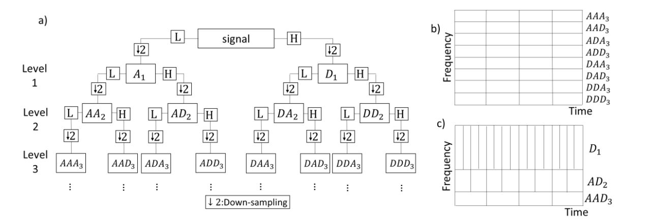
Approximation coefficient’s (ACs) and detail coefficient’s (DCs) of WPT (also of DWT) at each level are computed from the proceeding AC’s and DC’s using low-pass filters (i.e., H), high-pass filters (i.e. ,G), and decimation (i.e., ↓ 2) (Nason and Silverman 1995), as shown in Figure 1 (a). The low-pass filter has the coefficients of {h_n} in time-domain and they convolute with an infinite signal sequence {…, s₋₂, s₋₁, s₀, s₁, s₂, …} in time-domain:

When the sequence is finite, boundary conditions are applied at finite ends. Several different boundary conditions are available (Strang and Nguyen 1996) and periodic boundary condition is chosen in this study. Moreover, the filter coefficients should have a sum of squares equal to one (i.e., ${\sum }_n{h_n}^2=1$), and they should also satisfy the internal orthogonality condition:

The high-pass filter (G) coefficients (i.e., g_n) also obey the same rules and they are related to h_n:

Moreover, both filters satisfy the following mutual orthogonality relation:

These filters are determined by the wavelet type used in the composition. For down-sampling, binary decimator operator (i.e., D_o) chooses every even member of the sequence (shown as ↓ 2 in Figure 1 (a)):

Now, consider the signal sequence to be finite (e.g., s: s₀, s₁, …, s_N−1 where N = 2^J for some integer J). Consider that the signal equals to zero level approximation. AC’s and DC’s at other levels can be found:

where a and d are AC’s and DC’s, respectively, and the superscript on them denotes the decomposition level. The mapping of any sequence (e.g. s) to the pair of sequences (D₀Hs, D₀Gs) is an orthogonal transformation and therefore the filters are called quadrature mirror filters. At each level, the number of coefficients is reduced by 2.

However, DTW and WPT suffer from shift variance, which is a situation that a small shift of the signal can lead to large variations in the distribution of wavelet coefficients and therefore

resulting in changes in the reconstructed signal (Bradley 2003). The cause of shift variance is the down sampling of filter outputs, which violates Nyquist criteria and causes aliasing of frequency components above or below the cutoff frequency of the filter (due to the fact that an ideal filter is not achievable) into wrong decomposition levels.

One of the methods introduced to overcome this problem is SWT. First, to formulate SWT (Nason and Silverman 1995), ϵ-decimated Discrete Wavelet Transform (ϵDWT) is introduced. Define D₁ which is a binary decimation operator as D₀. However, D₁ selects every odd member of a sequence instead of the even member:

Now, define sequence ϵ: ϵ_J−1, ϵ_J−2,…, ϵ₀ as a sequence of 0’s and 1’s. Next, use the binary decimation operator $D_{{ϵ}_j}$ at level j to perform DWT. For each different ϵ, a different orthogonal transformation is obtained. DWT decomposed with different ϵ’s is referred as ϵDWT. It was shown that SWT includes every combination of ϵDWT (Nason and Silverman 1995). Therefore, the number of coefficients at each composition level of SWT equals to the number of signal points.

To directly obtain SWT transformation, DWT algorithm was modified. The modification was achieved by removing the decimation operators and padding zeros to high and low-pass filters at each level. To achieve the latter, define Z to be an operator that places zeros between each point of a signal so that (Zs)_2j = s_j and (Zs)_2j+1 = 0. Now, define filters H^[r] and G^[r] to be equal to Z^rh and Z^rg, respectively. Consequently, the coefficients of H^[r] equal to coefficients of H for every 2^rj’th coefficient, and to zero for the remaining 2^rj − N number of coefficients (i.e., $h_{2^{r}j}^{\left[r\right]}=h_j$, and $h_k^{\left[r\right]}=0$ if k is not a multiple of 2^r). Therefore, the following relationship holds:

Considering again that the signal equals to zero level approximation (a⁰ = s), AC’s and AD’s of SWT at other levels can be found:

References

• Bradley, A. P. 2003. “Shift-invariance in the Discrete Wavelet Transform.” Proc. VIIth Digit. Image Comput., 10–12.
• Nason, G. P., and B. W. Silverman. 1995. “The Stationary Wavelet Transform and some Statistical Applications.” 281–299. https://doi.org/10.1007/978-1-4612-2544-7_17.
• Strang, G., and T. Nguyen. 1996. Wavelets and Filter Banks. Wellesley: Wellesley-Cambridge Press.

• Wirsing, K. 2013. “Time Frequency Analysis of Wavelet and Fourier Transform.” Intech, 32 (July): 137–144.