Korkut Kaynardag
Multi-objective Optimization
I got into multi-objective optimization to update the model of a railway track. I ended up not performing this task due to time sensitive and more important tasks required for my project. However, I loved learning about multi-objective optimization and found it very fun. However, it was very challenging in the beginning. Therefore, here I wanted to explain briefly what multi-objective optimization is and what methods are used to solve it:
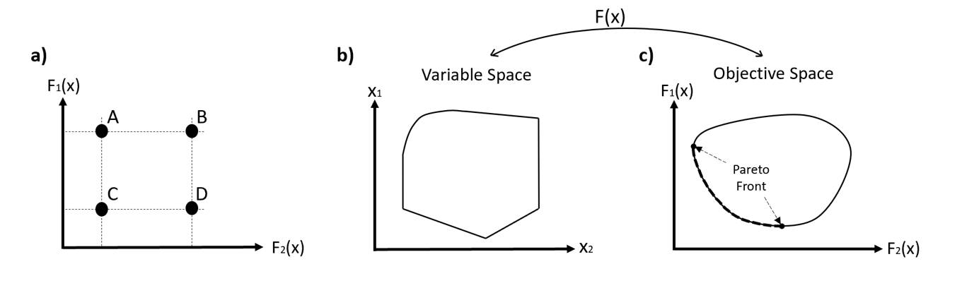
The simplest theory of multiobjective optimization is as follows: Let’s say we have 4 data points as a result of plotting our 2 objective functions (F1 and F2), as shown in Figure 1 (a). The goal is to find the point which is closer to zero (in this case, the point C).
However, in reality, the shape of the points is not as simple as it is shown in Figure 1 (a), and there can be more than 2 objective functions. Figure 1 (b) shows a representative space of variables that can be given to objective functions (2 variables are shown in this figure, but they can be more than 2 in reality). When these variables are given as input to objective functions, an objective space shown in Figure 1 (c) is obtained. The shape of this space is more realistic than the one shown in Figure 1 (a). The line denoted as Pareto Front on this figure is the set of Pareto efficient points. These points are determined based on the fact that none of the objective function values can be improved without degrading some of the other objective function values. The objective function values corresponding to the points that are not within the Pareto Front can be improved without degrading any other objective function value. Therefore, the points within Pareto Front are the most preferable solutions. Since there is not one possible solution, the decision-making process is involved in multi-objective optimization which makes it more challenging. The paper called “Multi-objective Optimization: Pareto Optimal Solutions, Properties” gives a very good introduction to multi-objective optimization and Pareto Front.
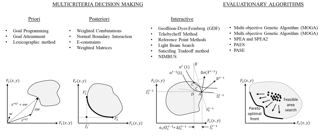
The algorithms to solve multi-optimization problems can be grouped as 1) Multicriteria Decision Making and 2) Evolutionary Algorithms (see Figure 2). The former can be grouped into three subgroups: 1) Priori methods 2) Posteriori methods and 3) Interactive methods. The explanation of Multicriteria Decision Making methods, the reason why evolutionary algorithms can perform better in solving multi-objective optimization problems, and a detailed explanation/comparison of evolutionary algorithms can be found in the paper called “Interactive Multiobjective Optimization: A Review of the State-of-the-Art”. Therefore, I suggest to the interested person to read this paper to learn more about these methods.
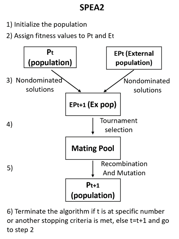
In Figure 3 that is illustrated below, I plotted the steps of SPEA2 method which si a widely adopted method to solve multi-objective optimization methods. The details of this algorithm can be found in the paper called “SPEA2: Improving the strength Pareto evolutionary algorithm”.