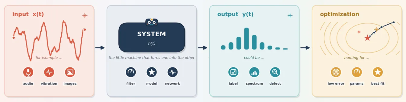
Signal Processing, System Identification, Estimation Theory and Optimization with the underlying logic of machine learning

In this section, I want to talk about signal processing, system identification, estimation theory, optimization, and how such topics establish the underlying logic of machine learning. As I mention on the home page, these subjects are all connected, because, to put simply, they mostly rely on the same underlying mechanism and solving that mechanism. Below, I first explain how these topics connect to one another, and then walk through the main methods and techniques that I have found most useful in each one.

I will also talk about the books that I think are most useful for each topic, including the math and probability background they draw on, since a solid foundation in probability and linear algebra matters a great deal here.

I hope you enjoy this section, and find it useful.

The Common Thread: Input, System, Output

As I understand it so far, signal processing, system identification, and machine learning are all built on one simple relationship: an input interacts with a system and produces an output (Figure 1). In most cases, optimization methods are what find the parameters of that system, the ones that make it produce the outputs we want.

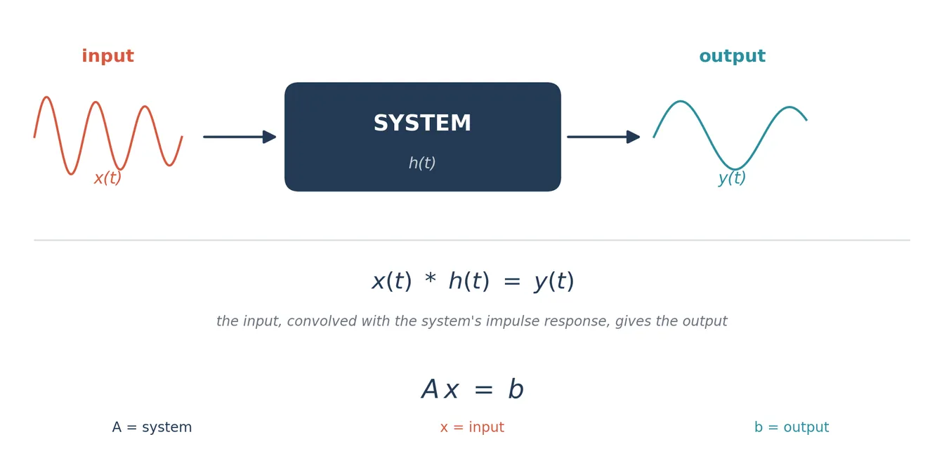
For example, signal processing methods usually require designing/finding filter coefficients. A non-neural network or a neural network-based machine learning (ML) method is to find the parameters and variables of the model that the system produces the outputs that we want. Optimization methods are what find those parameters. The goal of system identification, on the other hand, is to find the parameters of a system using only its output or using both its input and output. Again, optimization is what finds those parameters. So, depending on the application, the system in Figure 1 can mean different things: For example: in signal processing, it is usually the filter's coefficients; in machine learning, it is a neural network, for example one that performs image classification, or the parameters of some other machine learning model; and in system identification, it is the dynamic characteristics of a structure, a machine, or some other physical system (below, I explain in more detail what the system represents in different applications).

Now for the tricky part: system identification and signal processing can be difficult to tell apart sometimes due to 2 main reasons:

1. Some signals have specific features, particular frequencies, shapes, decay rates, phases, and so on, unless the signal is pure noise.. First, a signal can interact with a system and pick up that system's characteristics: wind blowing on a building will cause it to vibrate, and since buildings have specific resonance frequencies, a signal recorded from the building will carry the fingerprint of its vibrational behavior. Second, a signal can simply be generated with specific features to begin with, the way each word you speak creates acoustic waves with its own particular frequency content.

2. It is also useful to model signals that already have specific features as if they were the output of some hypothetical system, even when no such physical system really exists. Some examples are biological or financial time series, colored noise, and radar clutter.

The book Digital Signal Processing and Spectral Analysis for Scientists, by Silvia Maria Alessio, explains this approach clearly, and many signal processing books include a chapter on estimating the parameters of a signal, which really just means estimating the parameters of the real or hypothetical system that produced it. So, it is some kind of system identification approach, while it is stated as signal processing.

In my opinion, signal processing can be thought of as a form of system identification for a lot of applications, which is why I explain signal processing and system identification together below. I also go into more detail about what a system represents in different applications, and where optimization fits into the picture.

One note: even training a neural network can be thought of as a kind of system identification. In supervised learning, input-output pairs are used to determine a system, which is the trained network, that reproduces those outputs. Afterwards, the trained network is then used to predict the outputs for new inputs. I will explain this in more detail in the Machine Learning section below.

So, system identification really applies to signals that result from an interaction with a real physical system, but some approaches of signal processing work similarly for signals too (will explain below).

One more note: while system identification is the main core of vibration-based structural health monitoring (SHM), it is used from time to time in acoustic-based Non-destructive Testing (NDT). Generally, in NDT, especially ultrasound-based NDT, we send waves at specific frequencies with corresponding wavelengths, and can select their amplitudes and phases. To analyze such waves, usually system identification methods are not used (while sometimes they are used if the transmitted wave interacts with a defect and changes its properties too much, or to remove noise by correlating the input and output signals).

Signal Processing and System Identification

The most common uses of signal processing are 1) filtering a signal at specific frequencies, 2) extracting its frequency content, 3) enhancing particular features within signals, 4) reducing noise (meaning the unwanted signal component present in a measurement: this is done with filtering, but I will talk about a more advanced version, adaptive filtering, below), 5) and estimating the parameters of a signal, which is the part that overlaps with system identification. I will go over these below consecutively, while also explaining similarities to system identification.

When you filter a signal at specific frequencies, using a low-pass, high-pass, or band-pass filter (to remove the frequencies that you are not interested in), or a wavelet, which is used to see both when and at what frequency something happens in a signal, not just one or the other, letting you denoise, compress, and detect transients better than plain Fourier methods, the signal is being multiplied, in the time domain this is a convolution, with the impulse response of the filter or with the mother wavelet. So, this fits the same picture as Figure 1: the input is processed by a system, here, the filter's or wavelet's impulse response, to produce the desired output. We select/design these parameters based on our application.

If, instead, we look at features of the output signal, say, its dominant frequencies, that arose because the signal interacted with some system, we are doing system identification. For example, suppose a random signal interacts with a machine vibrating at some frequency you don't know, producing an output signal; taking the Fast Fourier Transform of that output will show a clear peak in the spectrum at the machine's vibration frequency. Real system identification problems are rarely this simple: they usually call for input-output methods, to cancel out the effect of the input when it isn't random, or output-only methods, to cancel out the effect of a random input. But the underlying picture is always the same, input, system, output, and that is what ties system identification and signal processing together.

You may also come across methods called template matching and matched filtering, whose goal is to detect or enhance a particular known signal buried in a noisy one. They work by correlating, essentially multiplying and summing, a known template signal against an unknown, noisy signal. In the language of Figure 1, the template plays the role of the system, the noisy signal is the input, and the output is the noise-reduced signal of interest.

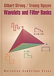
To learn about filters, parametric and non-parametric methods (will explain just below), and the basic idea behind wavelets, Digital Signal Processing and Spectral Analysis for Scientists is a very good book. To go deeper into wavelets specifically, Introduction to Wavelets and Wavelet Transforms: A Primer, by Burrus, Gopinath, and Guo, is an excellent, approachable introduction.

You will also hear a lot about parametric and non-parametric approaches when getting into signal processing or system identification, and for good reason, since the distinction comes up everywhere. In non-parametric methods, the goal is to estimate a signal's power spectrum directly from the data, without assuming any particular functional form for it, using methods such as the periodogram or the correlogram (which estimates the power spectrum from the signal's autocorrelation function). Because real signals are always finite in length, these estimates suffer from spectral leakage, where power at one frequency leaks into neighboring frequencies. In parametric methods, by contrast, the signal is assumed to be generated by a model with a known functional form, and the model's parameters are estimated from the data. Autoregressive (AR) modeling is probably the simplest and most common example of a time-domain parametric approach; ARMA and ARIMA models extend the same idea. Parametric methods can also be used to estimate missing segments of a signal, or to forecast its future values. And there are algorithms using this same parametric and non-parametric machinery to perform system identification, especially for vibration-based SHM. These are tailored, modified, and enhanced to handle multiple output channels (as in input-output experimental modal analysis), to remove or account for noise, to extract mode shapes and damping ratios, to track parameters that change over time due to nonlinearity, and to remove the effects of other variables, among similar tasks.

Before I learned these methods, I assumed they would be complicated and very different from one another. Once the core idea clicks, though, going deeper into parametric methods is genuinely easy and fun. Digital Signal Processing and Spectral Analysis for Scientists is, again, a really good book for getting into these approaches.

Ok, now let’s go step by step for a bit more and talk about adaptive filtering which is part of signal processing and also used in system identification:

About adaptive filters: Adaptive filters serve two main purposes, as far as I have seen: noise reduction and system identification. Either way, they need access to both an input signal and a desired output signal, and they update their own coefficients, sample by sample, using an optimization algorithm. The most widely used update rule is the Least Mean Squares (LMS) algorithm, which nudges the coefficients a small step in the direction that reduces the squared error; the Recursive Least Squares (RLS) algorithm is a more sophisticated, and faster converging, though more computationally expensive, alternative. There are also other algorithms to find the parameters.

To use adaptive filters for noise reduction, a reference signal, one that contains only the noise you expect to be present, is fed into the adaptive filter alongside the recorded signal (which contains both the desired signal and the noise you want to remove). The filter's coefficients are updated, using optimization, until the error between the filter's output and the desired signal is minimized; this works because the desired signal is uncorrelated with the noise reference. This only works, of course, when a suitable noise reference, correlated with the actual noise in the recording, is available. It is used a lot in acoustic noise reduction, where, confusingly, the desired signal is itself an audible sound, and the noise you are removing might be background noise or noise introduced by the recording instrumentation. So it is worth being precise about what you are calling noise in a given application.

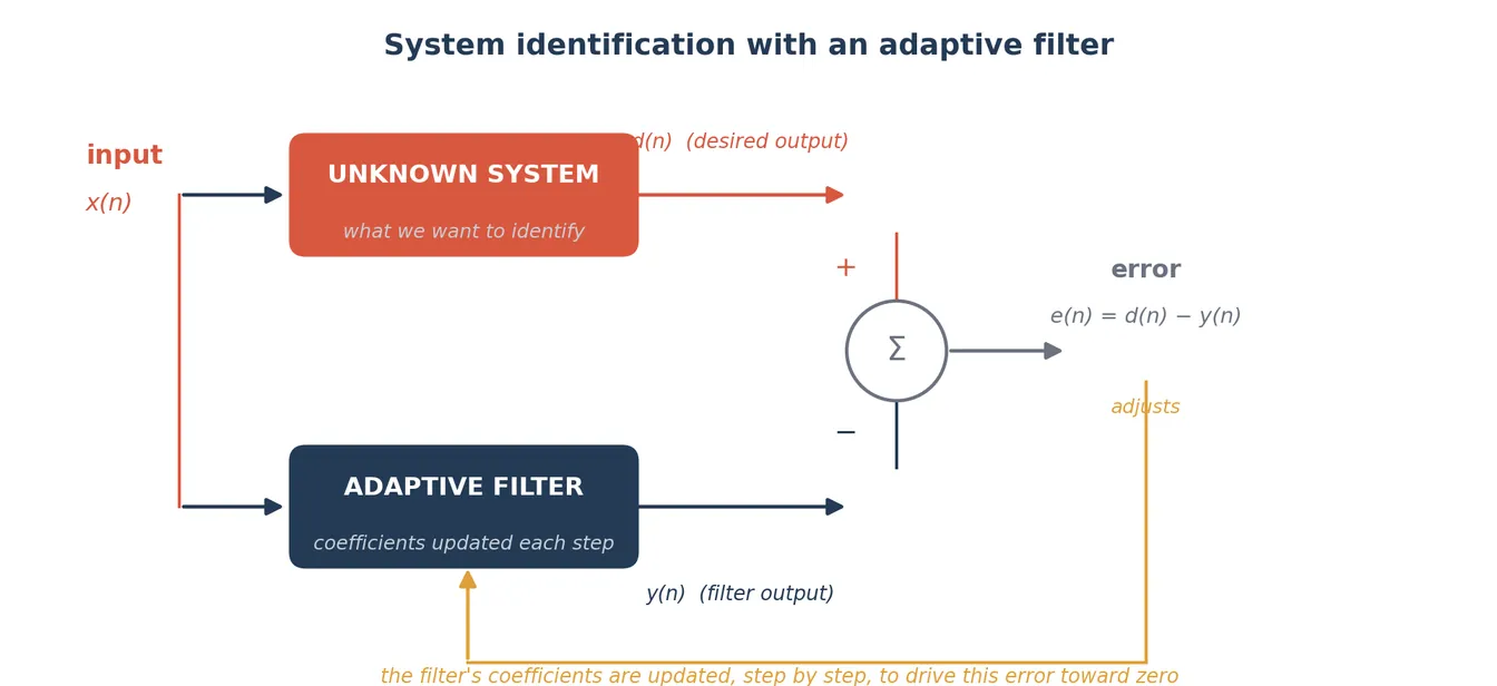
For the system identification application of adaptive filters, shown in Figure 2, the same input signal is fed into both the unknown system and the adaptive filter, and the filter's coefficients are updated until its output matches the unknown system's output as closely as possible. Once that happens, the filter's coefficients describe the characteristics of the unknown system. This is, in my opinion, the clearest bridge between adaptive filtering and both input-output system identification and machine learning (in both cases, we're recursively finding the model's coefficients or parameters using optimization, generally from input-output data). I'll talk more about this below. In addition, many system identification models using an adaptive filter approach exist in the literature.

Adaptive Filter Theory, by Simon Haykin, is a really good book for getting into adaptive filters properly, LMS, RLS, and beyond.

Here, my goal is to explain signal processing, and show its resemblance to system identification (which I believe also lets you learn the main idea of system identification along the way). Thus, I think I hit two birds with one stone. There are many system identification methods, which are usually more advanced, but I am not going into details of them here. Hopefully, in the future I'll make an introductory guide just for system identification used in SHM. There are also more different signal processing methods, but here I mentioned about the methods which lays the foundation of signal processing.

Estimation Theory

Now, let's talk about estimation theory. I want to do so because, when I first got into estimation classes and books, I expected them to be about estimating physical parameters of systems, frequencies, phases, mode shapes, that kind of thing. What actually confused me at first is that a signal can also be modeled purely statistically, as a random variable drawn from some probability distribution (a normal distribution with some mean and standard deviation, say), and estimation theory is just as much about estimating the parameters of that distribution as it is about estimating physical system parameters. But it is more than that!

A simple example that took me a while to really internalize what estimation theory is about: the familiar sample standard deviation formula is itself an estimator, in this case, an estimator of the dispersion of the underlying distribution. There are other estimators for the same quantity, some better than others depending on the situation, which is why the first homework sets in my estimation class, largely about estimating statistical parameters using different estimators, initially surprised and confused me.

Two core ideas come up constantly once you get into estimation theory. The first is maximum likelihood estimation (MLE), which picks the parameter values that make the observed data most probable under the assumed model. The second is least squares estimation, which picks the parameter values that minimize the sum of squared differences between the model's predictions and the observed data. When the measurement noise is Gaussian, these two approaches actually coincide. Least squares, in particular, is everywhere: it is, in a sense, the most common way of actually solving the $Ax=b$ problem from Figure 1 when there is noise in the measurements and no exact solution exists. Two more estimators are worth knowing. Maximum a posteriori (MAP) estimation is the Bayesian counterpart to MLE: it also picks the most probable parameter values given the data, but folds in a prior belief about the parameters too, it is directly related to regularization, since Tikhonov regularization is exactly MAP estimation with a Gaussian prior. The method of moments is older and simpler: it estimates parameters by matching the sample's statistical moments to the model's theoretical ones; it is less efficient than MLE in general, but cheap to compute, and is often used just to get a good starting guess for a more refined estimator.

This Wikipedia page has a good overview of the most commonly used estimators: https://en.wikipedia.org/wiki/Estimation_theory. You will find that the estimators listed there show up throughout signal processing, optimization, and machine learning books, as well as in books specifically about estimation.

Kalman filtering, something you will hear about constantly, is a widely used recursive state estimator, and it fits squarely under estimation theory: like MLE, least squares, and MAP above, it is ultimately about combining information optimally in the presence of noise. What makes it distinctive is how it does this, through two repeating steps. First, it predicts: using the system's dynamic model, it projects the current state estimate forward to the next time step, producing a predicted state and a predicted uncertainty (this uncertainty naturally grows during the prediction step, since the model itself is imperfect). Second, it updates: when a new noisy measurement arrives, the filter blends this prediction with the measurement, weighted by how much it trusts each one. If the measurement is noisy and unreliable, the filter leans more on its own prediction; if the measurement is precise, it leans more on the measurement instead. This weighting, called the Kalman gain, is computed automatically from the relative uncertainties (variances) of the prediction and the measurement, so at every step the filter is really just a running, confidence-weighted average between what the model expected and what was actually measured. The result is a new, blended estimate that is provably more certain than either the prediction or the measurement on its own, and, given noisy measurements of a linear dynamic system, this blended estimate is the statistically optimal estimate of the system's internal state, in the minimum mean-square-error sense, provided the process and measurement noise are well approximated as Gaussian.

Because it only needs the previous estimate and the newest measurement to produce the next one, rather than reprocessing the whole signal history, it is well suited to real-time applications. (For nonlinear systems, the same predict-update idea is extended through the Extended Kalman Filter and the Unscented Kalman Filter, which linearize the problem or approximate the relevant probability distributions.)

The Estimation Theory class that I took basically first covered the estimators, and then Kalman filter and its derivatives.

Stochastic Models, Estimation, and Control, by Peter S. Maybeck, gives a really good introduction to stochastic models, the basics of estimation theory and probability, and Kalman filters. This book helped me a lot in understanding these topics individually, and in seeing how they connect.

OK, A BIG CONNECTION PICTURE

I'm giving this to you before moving on to inverse problems, optimization, and machine learning, because I think this is exactly where the big picture comes together. So before going further, let's step back and look at the big picture while we have enough pieces in place.

It's worth spelling out how estimation connects to the Optimization section below, since the link is there throughout but never stated outright. Most of the estimators above are actually defined as the solution to an optimization problem: MLE is the parameter value that maximizes the likelihood, least squares is the parameter value that minimizes squared error, and MAP is the parameter value that maximizes the posterior. So computing an estimate, in practice, usually means solving an optimization problem, and an optimization algorithm is the tool that actually finds it. That said, estimation and optimization aren't quite the same thing: estimation asks what your best guess for an unknown quantity should be, and how good that guess is statistically (whether it's biased, how much it varies from sample to sample), while optimization is just the mechanism used to compute it. Not every estimator comes from an optimization problem, the method of moments above is one that doesn't, and not every optimization problem is an estimation problem either, minimizing a structure's weight subject to a strength constraint has nothing to do with estimating an unknown parameter from noisy data. But for the estimators that matter most in practice, MLE, least squares, MAP, and the Kalman filter, it's optimization doing the actual work underneath: each one is computed by solving an optimization problem, even though the result is reported and judged in the language of estimation theory (bias, variance, optimality) rather than the language of optimization

As explained above, estimation theory quietly sits underneath everything in this document, not just optimization. In signal processing, filtering, denoising, and parametric spectral estimation are all, at bottom, about estimating a signal's parameters, its frequencies, amplitudes, or the coefficients of a model like AR or ARMA, from noisy data; that's the estimation problem, stated plainly. In system identification, we never get to see a structure's or a machine's true resonance frequencies, damping ratios, or transfer function directly, we only get noisy measurements of its input and output, so identifying the system really is estimating its parameters from data, using the same MLE, least squares, or Kalman filtering machinery described above. And in machine learning, training a model is, again, an estimation problem in disguise: the true underlying function relating inputs to outputs is unknown, and training finds the parameters that best explain a finite, noisy training set, which is why so much of machine learning training quietly reduces to minimizing a loss function that is secretly least squares (mean squared error loss) or secretly MLE (cross entropy loss) in another form. So this is really the same picture as Figure 1, told a third way: signal processing, system identification, and machine learning are all, underneath, the same act of estimating an unknown system or its parameters from noisy data, and optimization is the shared mechanism all of them use to actually do it.

Here is a big table that shows the most commonly used methods, and whether each one relies on estimation theory, optimization, or both, to solve problems in signal processing, system identification, and machine learning. It also shows how the algorithms/methods/approaches used in signal processing, system identification and machine learning are connected and/or used in more than one of those fields. And this table is why you will see several topics in different books!

Inverse Problems and Regularization

Surprise: this isn't in the title, but I wanted to mention it anyway. Broadly, an inverse problem is about inferring an unknown cause, often the system itself, sometimes the input, from observed effects, the output. This is why inverse problems and system identification, and also machine learning overlap so much, and why optimization shows up here too: we are searching for the system, or input, that best reproduces the observed data. Inverse problems come up constantly outside structural or mechanical engineering as well; X-ray computed tomography and acoustic source reconstruction are two classic examples, among many others.

Many inverse problems are ill-posed, in the sense described by Hadamard: a well-posed problem has a solution that exists, is unique, and depends continuously on the data, meaning small errors in the measurements do not cause wild swings in the solution; an ill-posed problem fails at least one of these conditions, most often the last one. Regularization is the standard tool for taming ill-posed problems: it adds extra information or constraints, for example, a preference for smoother or smaller-magnitude solutions, as in Tikhonov (L2) regularization, to stabilize the solution. This is closely related to the idea of overfitting in machine learning: an unregularized model can chase the noise in the data as if it were signal, and regularization is what keeps it from doing that, so taming an ill-posed inverse problem and preventing overfitting really are two faces of the same coin.

This link is a good, visual introduction to underfitting and overfitting: link.

Therefore, I like to state that inverse problems and regularization are not a separate application in their own right, but are widely used in signal processing, estimation theory, system identification, optimization, and machine learning.

The best introductory book on inverse problems and regularization, in my opinion, is Parameter Estimation and Inverse Problems, by Aster, Borchers, and Thurber. It explains these topics with genuinely good explanations and visualizations.

Machine Learning

In machine learning, inputs and outputs are used to train a model, which, again, is just the system in Figure 1. Using the input-output pairs and an optimization method, we find the model (system) that best reproduces the observed outputs; once trained, the model can then be used to predict outputs for new inputs. This is really the same operating logic as adaptive filtering and system identification, so, once you have a decent grounding in signal processing, system identification, adaptive filtering, and optimization, machine learning is not a big leap. It's nothing scary!

Supervised learning: the model is trained on labeled input-output pairs, exactly the input-system-output picture above, and learns to map new inputs to predicted outputs. Classification and regression are the two big supervised tasks: classification assigns an input to one of a set of discrete categories (is this email spam or not?), while regression predicts a continuous numerical value (what will tomorrow's temperature be?).

Unsupervised learning: there are no labeled outputs at all, just inputs, and the goal is to find structure in the data on its own. Clustering, grouping similar data points together (k-means is the classic example), and dimensionality reduction, finding a simpler, lower-dimensional representation of the data (principal component analysis, for instance), are the two most common unsupervised tasks.

Both neural-network-based methods (generally called deep learning when many layers are used), and non-neural-network models exist. They can solve supervised and/or unsupervised learning problems. They can also do anomaly detection and forecasting. To understand those algorithms, when to use them, to what kind of data to use them, and their trade-off, please see my “Machine Learning - The Complete Picture and Guide” on my webpage, which explains machine learning in much more detail. Here, I only touched on it very briefly. That document will elaborately explain machine learning without extensive technical info.

Before ending the section, let me explain reinforcement learning as well, since it fits the input-system-output picture a little less directly than the others. Instead of learning a fixed mapping from a batch of labeled data, an agent interacts with an environment over time, takes actions, and receives rewards or penalties, and it learns a policy, a strategy for choosing actions, that maximizes its cumulative reward. It is closer to an optimal control problem than to a regression problem, but the same underlying optimization machinery, gradient-based methods especially, is usually what trains it.

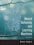
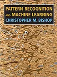
In my opinion, Neural Networks and Learning Machines, by Simon Haykin, who also wrote Adaptive Filter Theory, is a very good book for getting into machine learning; it is no accident that the same author wrote both, since, as I mentioned above, I think of machine learning as very much a continuation of adaptive filtering. For deep learning specifically, Deep Learning, by Goodfellow, Bengio, and Courville, and Pattern Recognition and Machine Learning, by Christopher Bishop, are excellent next steps.

Optimization

Optimization problems are usually described along a few independent characteristics: (i) whether the objective function (and feasible region, if there are constraints) is convex or nonconvex; (ii) whether the objective function and constraints are linear or nonlinear; (iii) whether the problem is constrained or unconstrained; and (iv) whether we are looking for a local optimum or the global optimum.

It is worth being precise about how these characteristics relate to each other, since I got this wrong myself for a while when I was starting out. Convexity and linearity are not the same axis: a problem can be linear and convex, nonlinear and convex, or nonlinear and nonconvex. Linear programs, meaning problems with a linear objective function and linear constraints, are, in fact, always convex; they are really the simplest and most well understood class of convex optimization problem, not an exception to it. Nonlinear problems, on the other hand, can go either way: a nonlinear objective function can still be convex (a convex quadratic function is a common example), or it can be nonconvex, which is the case for most neural network training problems, and for many other nonlinear least-squares and physics-based fitting problems.

The reason convexity matters so much is that a convex problem has a single, wonderfully convenient property: every local minimum is automatically the global minimum. So for convex problems, a local optimization algorithm, one that just follows the local slope downhill, is guaranteed to find the actual best solution. Nonconvex problems don't offer this guarantee: they can have multiple local minima, and a local algorithm can easily get stuck in one that is not the global minimum. Figure 3 illustrates the difference. Both linear and nonlinear optimization problems, convex or not, can be constrained or unconstrained. This webpage has a nice visualization of linear versus nonlinear programming specifically: link.

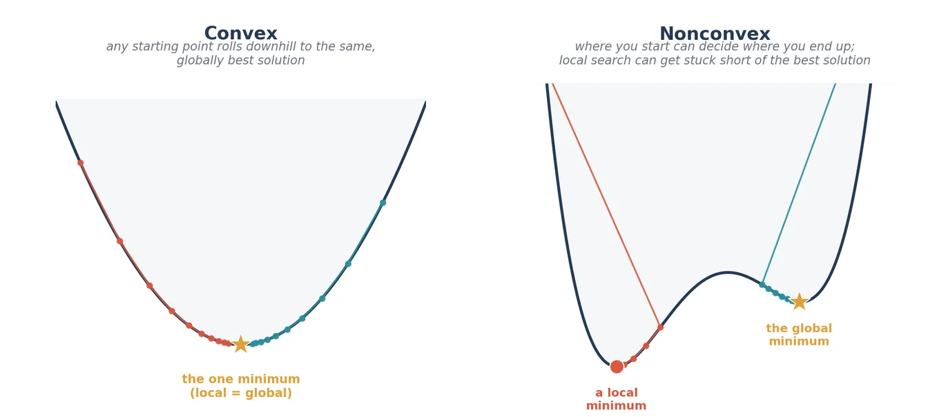
Accordingly, algorithms for solving optimization problems are usually grouped into local and global optimization algorithms. Local algorithms are generally gradient-based (a few non-gradient local methods exist too), meaning they use the local slope, and sometimes curvature, of the objective function to move toward a nearby optimum. To handle constraints with a local algorithm, the constrained problem is usually first converted into an unconstrained one, most often by folding the constraints into the objective function as penalty terms. The local optimization algorithms you will run into most often in signal processing and machine learning books are Newton's method (which also uses curvature information and converges very fast near the optimum, but is expensive for problems with many parameters), Gradient Descent, Conjugate Gradient Descent, and Stochastic Gradient Descent, the workhorse of most neural network training, where the gradient is estimated from a small random batch of data at each step rather than the full dataset.

Global optimization algorithms are used when a problem is expected to have multiple local minima and the goal is to find the global one. These are usually grouped into evolutionary and other, more deterministic, global methods; evolutionary algorithms, inspired by processes observed in nature (and, yes, sometimes given fittingly playful names), are the ones you will encounter most often. They work by evolving a whole population of candidate solutions toward the global optimum, generation by generation, rather than following a single point downhill. The most common examples you will see in the literature are the Genetic Algorithm, Particle Swarm Optimization, Simulated Annealing, and Ant Colony Optimization. Because they do not rely on gradient information, they can be used even when the objective function is non-differentiable, discontinuous, or only available as a black box, situations where gradient-based local methods cannot be applied at all.

For a nice, brief overview of local and global optimization algorithms, the paper “A Review of Optimization Techniques” is a good place to start. For a much more detailed review of gradient-based local optimization algorithms specifically, this page is excellent: https://ruder.io/optimizing-gradient-descent/.

Optimization problems can also have more than one objective function at once, leading to multi-objective optimization. Rather than a single best answer, this usually produces a whole set of trade-off solutions, called the Pareto front, where improving one objective necessarily makes another one worse, and no single solution dominates all the others across every objective. Please see my blog for more on multi-objective optimization; having more than one feasible, non-dominated solution to choose from makes these problems more challenging, but also, in my opinion, more fun to work through.

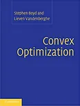
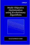
Convex Optimization, by Stephen Boyd and Lieven Vandenberghe, is, by a wide margin, the best book for really understanding convexity and convex optimization. Nonlinear Optimization, by Andrzej Ruszczyński, is a good next step into the broader nonlinear (convex and nonconvex) landscape, and Multi-Objective Optimization Using Evolutionary Algorithms, by Kalyanmoy Deb, is an excellent, focused treatment of multi-objective problems and the evolutionary algorithms used to solve them.

Blind Source Separation

One topic I have not mentioned yet, but that fits the same picture as everything above, is blind source separation (BSS). Its classic motivating example is the cocktail party problem: you are recording several microphones' worth of audio at a party, and each microphone picks up a mixture of everyone talking at once; the goal is to recover each individual person's voice from the mixed recordings, without knowing, in advance, how the voices were mixed together, hence blind.

In the language of Figure 1, the unknown mixing process is the system, the individual source signals are the input, and the mixed microphone recordings are the output; BSS is the inverse problem of recovering the input, and, implicitly, undoing the system, from the output alone, which is why I think of it as sitting right alongside system identification and inverse problems, rather than as some completely separate topic. The most common approach is Independent Component Analysis (ICA), which assumes the original sources are statistically independent of one another, and uses that assumption to find an unmixing matrix that separates the mixed signals back into their original, independent components.

Blind Source Separation: Theory and Applications, by Yu, Hu, and Xu, is a solid introductory book on this topic.

Closing Thoughts

It took me about 8 years of grad school to piece together the picture I have tried to lay out in this section, so take your time with it, and try to enjoy the process of learning.

1. Everything above, in my opinion, can be boiled down to $Ax=b$, where $A$ is the system, $x$ is the input, and $b$ is the output, a framing I picked up from one of Stephen Boyd's lectures (he is also the coauthor of Convex Optimization, mentioned above). If you can write a problem in this form, and can solve it, minimizing the effect of noise when the measurements are noisy, you can, in principle, solve a remarkable range of problems in signal processing, system identification, and machine learning. So, in a sense, it really does all come down to $Ax=b$.

2. as you read this document, I hope that, you understood how many topics are connected to each other. In my opinion, if you have a good foundation and understanding of the topics mentioned here, you will start to understand many research papers and algorithms on these topics, and learn the more complex ones easily. And, now you will also understand, why same topics and/or sections are explained in many different books and topics.

3. To learn system identification (which is one of my research topics): as a civil engineer, most of my own work has involved identifying structural systems, meaning their resonance frequencies, mode shapes, and damping ratios. As I explained above, system identification really is a big part of signal processing, so a solid grounding in signal processing, the basics of optimization, and some probability is genuinely necessary before getting into system identification specifically. In particular, I would make sure to understand digital filters, wavelets, parametric and non-parametric spectral methods, Bayesian methods (which I have not covered above, but which are a widely used framework for statistical inference), some optimization methods such as gradient descent, the basics of estimation theory, adaptive filters, and the basics of inverse problems. With that foundation, learning system identification methods from books or papers becomes much easier.

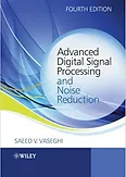
4. To go deeper into probability, Bayesian methods, and stochastic processes, I have found the following books useful: Advanced Digital Signal Processing and Noise Reduction, by Saeed Vaseghi; Stochastic Processes: Theory for Applications, by Robert Gallager; and Random Data: Analysis and Measurement Procedures, by Bendat and Piersol. The system identification books I would recommend most are System Identification: Theory for the User, by Lennart Ljung, and Linear Systems Theory, by João Hespanha.

The Books

Below, I have grouped the books I have found most useful into eight categories: signal processing, optimization, wavelets, stochastic processes and random data, system identification, inverse problems, machine learning, and blind source separation. This grouping is based on each book's main focus, but, as I mentioned above, the topics themselves overlap a great deal; probability, some math, signal processing, estimation methods, and even some optimization methods show up in a large fraction of these books, regardless of which category they are filed under.

Because of that overlap, I would recommend reading one or two books from each category to get a well-rounded picture of how signal processing and system identification, optimization, and machine learning fit together. Within each category, I have tried to list the best introductory book first; the books listed after it are good follow-ups once you want to go deeper into the theory.

I hope the books listed here, together with my explanations above, give you a useful, overall picture of these fields.

Signal Processing

Optimization

Wavelets

Stochastic Processes and Random Data

System Identification

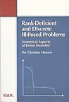
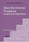
Inverse Problems

Machine Learning

Blind Source Separation