Dynamical Behavior of Engineering Structures and Acoustic Wave Propagation

In this section, I want to talk about structural vibrations and about acoustic waves propagating in solids. (Sound waves propagating in air, and how they can be used to track down a source that is emitting sound, are covered separately in the My Research section of this webpage.)

I will also explain how all vibrations are actually due to wave propagation. This is something I touched on briefly in the Structural Health Monitoring (SHM) and Nondestructive Testing (NDT) part of my Research section; here, I want to expand on it more.

At the end of this section, I will list the books that I consider most useful for learning structural dynamics and wave propagation. As usual, everything explained here is based on my own knowledge, understanding, and experience.

Structural dynamics and wave propagation connect civil engineering, structural health monitoring (SHM), and nondestructive testing (NDT) to a wide range of phenomena in nature and everyday life through shared principles such as oscillation, resonance, interference, reflection, scattering, and energy transfer.

This makes learning vibrations and wave propagation in solids a part of a broader scientific approach that combines physical modeling, sensing, signal processing, and inverse problems to understand complex systems without taking them apart.

I hope you will enjoy this section but see the fun table below before diving into document:

Category	Schematic figure	Connection and explanation
Structural dynamics	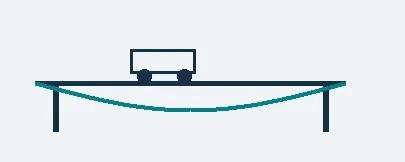Bridge vibration	Traffic excites bridge vibrations. Natural frequencies and mode shapes depend on mass, stiffness, and support conditions. Earthquake engineering calculates the responses during a seismic event, while SHM tracks changes in these responses, while accounting for temperature and loading.
Music and acoustics	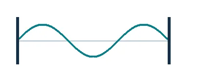Vibrating string	A guitar string supports standing waves and resonant modes, much like beams and cables. Changes in tension, mass, or stiffness alter its frequencies, the same physical sensitivity used in vibration-based monitoring.
Fluid mechanics	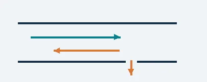Pressure-wave reflection	Pressure disturbances travel through pipes and reflect from changes in hydraulic conditions. Their timing and shape can help locate leaks, much as elastic-wave reflections help locate defects in solids.
Seismology and acoustic emission	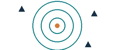Source location	Earthquakes and local cracking release elastic waves. Arrival times at several sensors help locate the source. Acoustic emission applies this idea to damage events in structures, at much smaller scales.
Optical fibers	Guided light	Optical fibers guide electromagnetic waves; plates, rods, and rails guide elastic waves. Both support propagation modes shaped by geometry and boundaries. Fiber-optic sensing also enables structural strain measurements.
Quantum mechanics	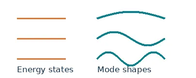Discrete states / modes	Discrete quantum energy states have mathematical parallels with structural vibration eigenmodes. Both fields also involve interference and scattering. In this case, a quantum wavefunction represents probability amplitudes, not structural displacement.
Electromagnetics	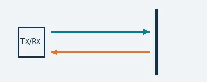Radar reflection	Radar waves reflect and scatter at changes in electromagnetic properties. Ground-penetrating radar investigates concrete and subsurface interfaces, much as ultrasonic NDT uses elastic waves to investigate mechanical discontinuities.
Lasers and optics	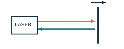Noncontact vibration sensing	Laser vibrometers use optical interference and the Doppler effect to measure surface motion without contact. Laser pulses can also generate ultrasound, directly connecting optical methods with structural dynamics and NDT.
Medical ultrasound, sonar and echolocation	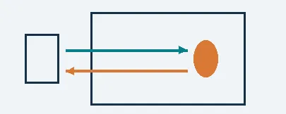Pulse and echo	Medical ultrasound, sonar, and bat echolocation use returning sound waves to reveal interfaces or locate objects. Ultrasonic NDT similarly interprets travel time, amplitude, and waveform changes to investigate internal features.
Electrical circuits	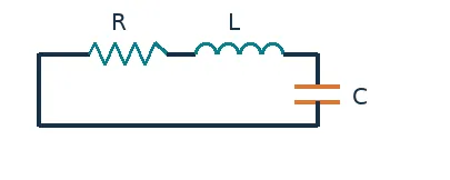RLC and mechanical resonance	Resistor–inductor–capacitor circuits and mass–spring–damper systems share second-order mathematical models. Both exhibit resonance, damping, and frequency-dependent response, enabling similar analysis and identification tools.

Conceptual schematics. Shared mathematical ideas do not imply identical physical mechanisms.

Conventional Structural Dynamics and Vibration based SHM

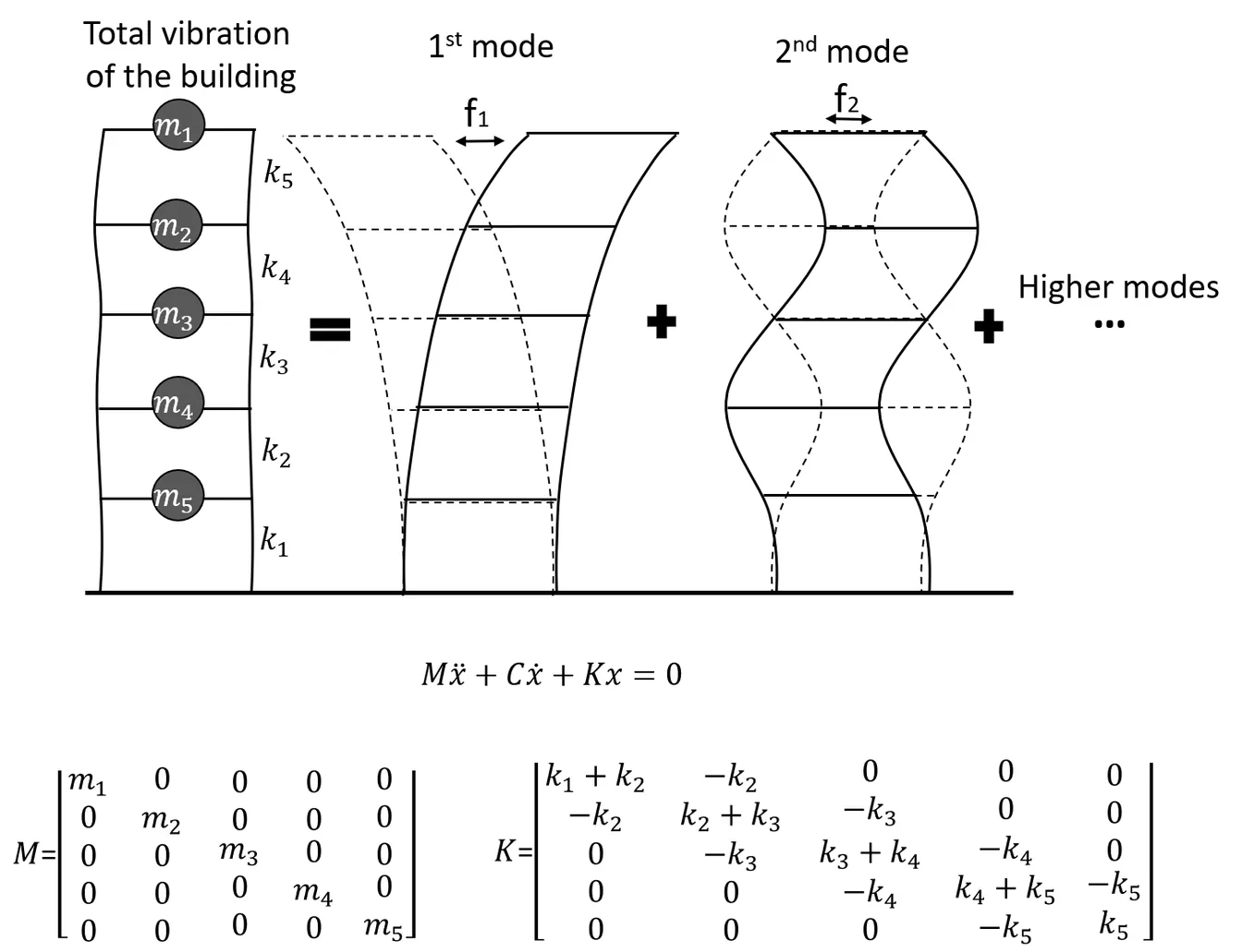
In structural dynamics and earthquake engineering courses, we are taught to model structures using discretized versions of what are actually continuous systems. Figure 1 shows the discretized dynamic model of a building, used to analyze its lateral natural vibration modes and shapes: masses and stiffnesses are assigned at each story, treated as lateral degrees of freedom. Doing this lets us write the equation of motion using discretized mass and stiffness matrices (shown below the figure), from which we can find the eigenvalues, which are the resonance frequencies, and the eigenvectors, which are the mode shapes. Usually, we only care about the first few resonance frequencies, and these tend to be low, under about 10 to 20 Hz for most structures. Very stiff structures are an exception: a rail beam connected by two fasteners, for example, can have a first mode around 1 kHz because of its very high stiffness. But generally, the first few modes of buildings, bridges, towers, and similar structures fall under approximately 10 to 20 Hz. In vibration based SHM, these dynamic parameters are identified and tracked over time for condition assessment. It is kind of straightforward: because these parameters describe the structure globally, they are good at revealing its overall condition. If the mode shapes are measured with enough spatial resolution, which depends on how many measurement points are placed on the structure, local changes in the mode shapes can even help locate damage. However, the exact location of a crack, the size of a delamination, and other detailed defect properties cannot be identified this way with much accuracy. This is where acoustic wave-based NDT comes in.

Why Resonance Happens: Interference of Travelling Waves

However, these low frequency global vibration parameters of structures (for example, the resonance modes) are actually caused by propagating waves, as I introduced in the SHM and NDT part of my Research section. Here is how it happens: waves whose half wavelength divides evenly into the length of the structure (say, a simply supported beam) can propagate along it with much less attenuation than waves whose half wavelength does not. This is because reflections from the boundaries send waves travelling in two opposite directions at once, and where their half wavelength fits the span, these two waves interact constructively. That constructive interaction is what creates a standing wave, and a standing wave is exactly what we call a resonance mode of the structure. Discretized modeling is simply a convenient way to get to the same answer: the frequencies and mode shapes of these standing waves, that is, the resonance modes, can be obtained easily this way, and the resulting equations can also be solved with the Finite Element Method, since they are already discretized.

The figure below (Figure 2) helps visualize why resonance frequencies occur, as a result of wave propagation. Figure 2 (a) shows a specific type of wave, a flexural (bending) wave, propagating on an infinitely long beam. Suppose these waves are induced by an excitation with broadband frequency content (see Figure 2 (b)), meaning it contains energy across a wide range of frequencies at once, like an impact. As a result, waves at many different frequencies all propagate freely on the infinite beam. If we then measured the beam's dynamic response after the impact, at any point, using accelerometers, and computed a frequency spectrum from the recorded data, we would get something like the flat spectrum shown in Figure 2 (b). Now suppose instead that we have a finite beam, as in Figure 2 (c). Its frequency response would look like Figure 2 (d), provided the measurement is taken some time after the impact; it would only resemble the flat spectrum of Figure 2 (b) if the measurement were taken immediately after the impact. The reason is that, as time passes, waves at frequencies away from resonance attenuate much faster than waves at the resonance frequencies. Therefore, the longer we wait between the impact and the measurement, the more the non resonant peaks fade relative to the resonant ones. Eventually, all the waves die out due to damping. But the key point is that, for a while, the waves at the resonance frequencies dominate the response.

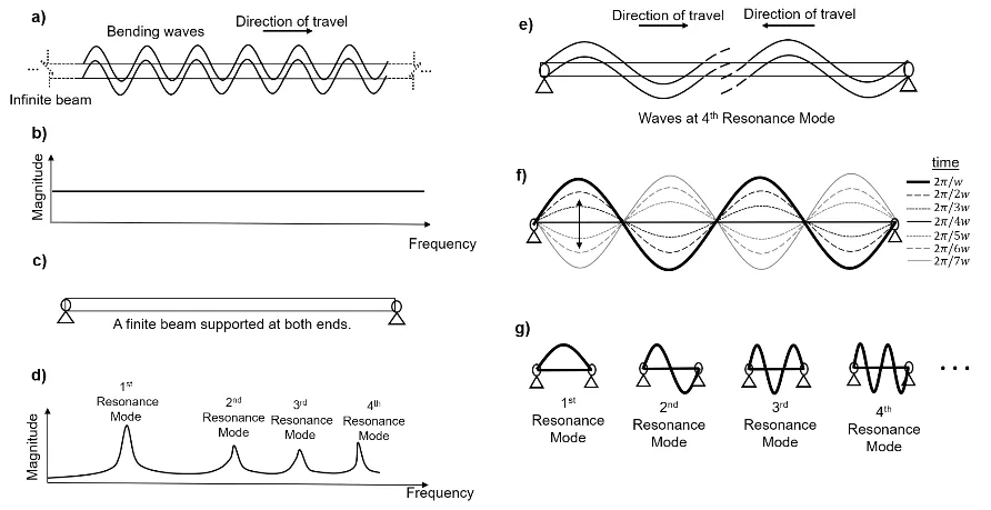
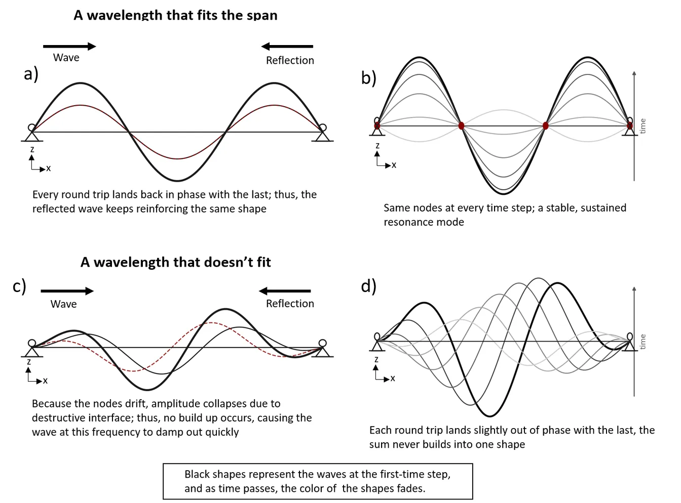
So, what happens to waves at the non-resonance frequencies? Why can't they propagate as easily as waves at the resonance frequencies? The reason is that the interference between these waves is messy, and the wave energy dies out quickly because the interaction is mostly destructive: the wave travelling in one direction and the wave reflected back in the opposite direction do not line up, so instead of reinforcing each other, they largely cancel out. I will reuse a figure I made for the my research section documents in this webpage, since I really like it. Figure 3 (a) and (b) show how a standing wave forms a resonance mode when the reflected waves interact constructively. As time passes, this standing wave still decays, but only because of damping in the beam (see Figure 3 (b)); the shape of the mode itself, the standing wave pattern, does not change. By contrast, Figure 3 (c) and (d) show what happens at a frequency whose half wavelength does not fit evenly into the length of the beam: the random interference between the reflected waves is mostly destructive, so the waves attenuate much faster, on top of the attenuation from damping. And as time passes, the shape of this non resonant interference pattern keeps changing, unlike the fixed shape of the standing wave, and it dies out faster too.

Wave Propagation in a Beam with More Depth: Dispersion Curves

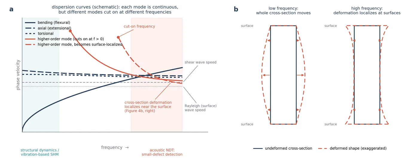
Now, let's consider wave propagation in a beam in more depth. As frequency increases, the number of waves that can propagate at once increases, and the cross sectional deformation of these waves becomes progressively more complex. At lower frequencies, the entire cross section deforms together, for example through bending, torsional, or axial motion, while at higher frequencies the deformation of a wave can localize at specific parts of the cross section, as happens with surface waves. Dispersion curves, a term you will hear a lot once you get into wave propagation, show how a wave's speed, or equivalently its wavelength, varies with frequency. Figure 4 (a) illustrates this schematically: each curve, or mode, is continuous across all frequencies. But different modes with their own characteristic cross-sectional deformation start, or “cut on,” at different frequencies. As frequency increases, modes with more complex, and eventually more localized, cross-sectional deformation begin to propagate. Figure 4 (b) contrasts a low frequency mode, whose deformation spans the entire cross section, with a high frequency mode, whose deformation concentrates near the surfaces. Accordingly, bending, lateral, and torsional waves start at the lowest frequencies, while more localized waves, surface waves being one example, only start at higher frequencies. Thus, while lower frequencies are used in vibration based SHM, higher frequencies are used in wave based NDT.

However, as I explain below, when a structure is restrained at both ends, only waves with specific wavelengths can propagate as standing waves. In many cases, a discretized equation of motion (that is, a standard finite element model of the whole structure) is enough to obtain the frequencies and shapes of these waves, in other words, the resonance frequencies and mode shapes, especially since structural dynamics, earthquake engineering, and vibration based SHM are usually concerned with the lowest order bending, lateral, torsional, and axial behavior. Dispersion curves, on the other hand, are essential when acoustic based NDT is used, because higher frequency, more localized waves are needed to detect small defects.

There are two approaches to obtaining dispersion curves: one is purely analytical, and the other is the semi analytical finite element (SAFE) method. (Do not let the name scare you: it once scared me too, when I first started learning wave propagation. It is actually quite simple.)

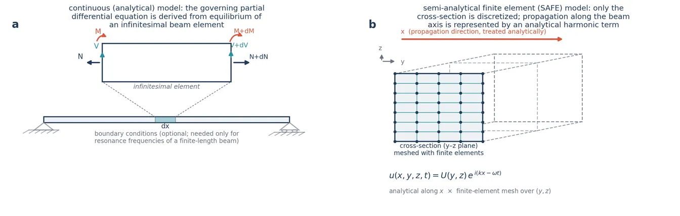
In the analytical approach, the structure, a beam in our case, is modeled as a continuum, and its governing equation of motion is derived from the equilibrium of an infinitesimal element of the beam (see Figure 5 (a)). Boundary conditions can be added to this equation to obtain the resonance frequencies of a finite length beam, but it is just as common to leave them out and solve for the dispersion curves of an infinitely long waveguide instead.

The analytical approach works well for simple, canonical cross sections, such as rods, beams, or plates, whose governing equation can be written and solved in closed form. For more complex or arbitrary cross sections, the semi analytical finite element (SAFE) method is used instead (Figure 5 (b)). Therefore, analytical formulations are usually good for modeling wave propagation at lower frequencies. In SAFE, only the cross section of the structure is discretized with standard finite elements, exactly as in ordinary structural finite element analysis, while propagation along the length of the structure is still treated analytically, through an assumed harmonic wave term of the form . Substituting this assumed form into the finite element equations of the cross section turns the three dimensional wave propagation problem into a two dimensional eigenvalue problem: for each frequency, or wavenumber, solving this eigenvalue problem returns the wavenumbers, or frequencies, that can propagate, together with the eigenvectors that describe the cross sectional deformation, that is, the mode shape, of each wave.

After the equation of motion has been formulated, whether analytically or through SAFE, the frequencies and shapes of the waves that can propagate on the structure are found using its boundary conditions: where these waves reinforce each other, they form standing waves, and this is where resonance frequencies come from. But usually, the goal when using FEM in an NDT study is to obtain waves propagating at higher frequencies, since they are sensitive to small defects and reflect due to their very small wavelength and localized cross sectional deformations. If the structure is also effectively infinitely long, for example a long plate, beam, or similar waveguide, its dispersion curves can be obtained from the same governing equation, again without imposing boundary conditions.

What Happens then in Periodically Supported and Multi Span Beams?

I explained above how wave propagation creates the resonance frequencies and mode shapes of a simply supported beam. Now, what if the structure is a periodically supported, infinitely long beam? This is the case where neither the pure structural dynamics approach (based on resonance frequencies and mode shapes) nor the pure wave propagation approach applies on its own. In my opinion, that is because structural dynamics and wave propagation get combined for this case. I will explain this below. Afterward, I will talk about the dynamics of finite multi span beams. Then I will use the vibration behavior of rails to wrap up my explanation of wave propagation and structural dynamics, including the cases where neither approach can be used on its own. Rail is a great example for this, since it is essentially an infinitely long, periodically supported beam with a complex cross section.

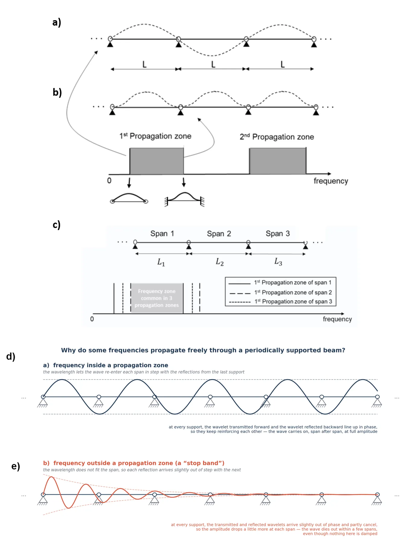
Let's start with an infinitely long, periodically supported beam. In such beams, waves with frequencies in specific ranges, called propagation zones, can propagate freely, because their wavelength satisfies the boundary conditions at every support. Waves whose frequencies fall outside these ranges attenuate quickly, since they cannot satisfy the support conditions; as I explained above, this attenuation comes from destructive interference caused by reflections from the supports, and is different from attenuation due to damping. There turns out to be a direct relationship between the bounding frequencies of the propagation zones and the resonance frequencies of finite beams: (i) the starting frequency of the Nth propagation zone corresponds to the Nth resonance frequency of a finite beam that has the same support conditions, at both ends, as the periodically supported infinite beam, and (ii) the ending frequency of the Nth propagation zone corresponds to the Nth resonance frequency of a finite beam with fixed fixed supports. As an example, Figure 6 (a) shows two waves that can propagate freely on an infinitely long beam periodically supported by pins; these two waves correspond to the first vibration mode of a simply supported span and of a fixed fixed span, respectively. Figure 6 (b) shows a representative spectrum with the first and second propagation zones marked. The paper “Wave propagation and natural modes in periodic systems: I. Monocoupled systems” explains this phenomenon nicely.

In reality, the span length and the forces applied by the connections are usually not identical from span to span, due to manufacturing imperfections. These imperfections give each span slightly different dynamic properties, so each one ends up with a similar but slightly different propagation zone. Because of this, several studies have looked at the dynamic behavior of infinitely long, nearly periodic beams. To see what happens, consider three consecutive spans of different lengths in an infinitely long, nearly periodic beam, labeled span #1, #2, and #3, as shown in Figure 6 (c), along with their first propagation zones. As the figure shows, each span has a slightly different propagation zone. Only waves whose frequency falls within the zone common to all three spans can propagate freely along all three; waves whose frequency falls outside that common zone attenuate due to reflections from the supports.

Figure 6 (d) shows a propagating wave whose frequency is within the first propagation zone while Figure 6 (e) illustrates a wave whose frequency is outside a propagation zone, hence attenuating faster than the wave in Figure 6 (d). Accordingly, Figure 6 (d) also illustrates the earlier point about propagation zone boundaries: the frequency of this wave is neither the resonance frequency of the pin pin span nor of the fixed-fixed span, but somewhere between them, which is exactly why it still propagates freely.

Here, I tried to introduce this phenomenon with the simplest explanation possible. As you go deeper into papers studying propagation zones in periodically or nearly periodically supported beams, you can get into much more detail, if you are curious.

But what about finite beams with multiple supports? Consider a multi span beam with three identical spans. What happens is that the first three resonance frequencies of the multi span beam fall within the first propagation zone of a periodically supported, infinitely long beam with the same span length; the next three resonance frequencies fall within the second propagation zone, and so on. The papers “Natural flexural waves and the normal modes of periodically supported beams and plates” and “Free wave propagation in periodically supported, infinite beams” explain this phenomenon very nicely.

However, things get more interesting once the span lengths are not identical. Let me walk through two illustrative examples, using approximate frequency values from experience rather than an actual computation.

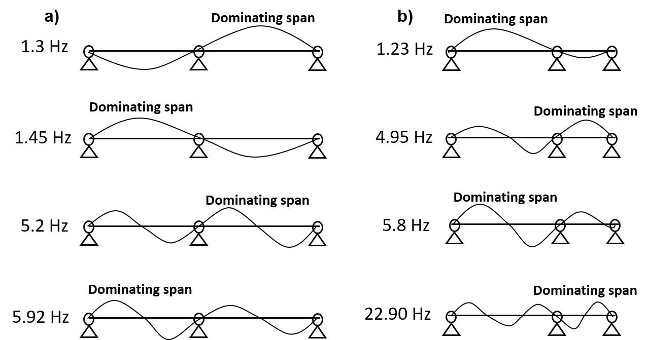
Consider a two span beam where the two spans have similar, but not identical, lengths. Uncoupled, that is, if each span were its own independent simply supported beam, their first two natural frequencies would be around 1 and 5 Hz for one span and around 1.2 and 5.7 Hz for the other. Once the two spans are joined into a single continuous beam, these shift into a new set of coupled natural frequencies for the whole system: something like 1.3, 1.45, 5.2, and 5.92 Hz (Figure 7 (a)).

Now consider a second two span beam where the spans have very different lengths, so their uncoupled frequencies are much further apart: around 1 and 5 Hz for the longer span, and around 4.6 and 21.3 Hz for the shorter one. Once connected, the coupled frequencies of this beam come out around 1.23, 4.95, 5.8, and 22.90 Hz (Figure 7 (b)).

In both cases, each of the four coupled mode shapes is dominated by whichever span's uncoupled frequency lies closest to it: that span deforms with something close to its own natural mode shape, while the other span is simply forced to go along with it through the shared support.

But the shape the non dominating span takes on is not arbitrary. It is whatever shape that span would naturally take if a wave at this frequency were forced onto it. Accordingly, the shape in the other span resembles whichever of its own modes has a natural frequency closest to that value, though not exactly, since it is being forced rather than resonating freely. This is why the two cases look different. In Figure 7 (a), the spans are similar in length, so their natural frequencies sit close together mode for mode; at any of the four coupled frequencies, both spans end up close to the same mode number, so the non dominating span's shape looks similar in form to the dominating span's (both single hump, or both double hump). In Figure 7 (b), the spans are very different in length, so their natural frequencies are spread far apart. At 22.90 Hz, for example, the shorter span sits right at its own second natural frequency and dominates with a two hump shape, while the longer span, whose own frequencies are much lower, is actually closer to one of its higher order modes at that same frequency, so it ends up with a shape that has more humps than the span that governs the overall mode.

So, the resonance frequencies and mode shapes of finite, multi span beams are governed by wave propagation too, which makes sense, since all vibration ultimately comes down to wave propagation. The paper “Vibration characteristics analysis of disordered two-span beams with numerical and experimental methods” provides a detailed vibrational analysis of a two span beam along these lines.

Case Study: Wave Propagation in Rails (infinitely long periodic beams)

Now let me use the rail as a worked example, to help visualize everything I explained above. Figure 8 (left) shows the dispersion curve of a rail, treated as infinitely long with no supports. As you can see, as frequency increases, the number of waves that can propagate at once increases. Up to around 25 kHz, the cross sectional deformation of these propagating waves is global, meaning the whole cross section deforms together. This dispersion curve was obtained using the semi analytical finite element method. This is because purely analytical methods can only model rail dispersion curves up to about 4 or 5 kHz (since analytical models have relatively few degrees of freedom), so they can only capture a handful of waves with simple cross sectional deformations. Figure 8 (right) shows a bending wave propagating in a rail that is periodically supported by fasteners. Because of this periodic support, the wave can only propagate within specific propagation zones, exactly as I explained above. If the rail were instead supported by just two fasteners, one at each end, rather than periodically and infinitely, only the waves that create its resonance frequencies could propagate. The spectrum in the lower part of the figure (a representative spectrum, not one obtained from an actual computation) illustrates the propagation zones for these bending waves.

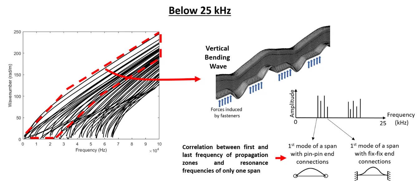
Note: here I only showed the bending waves. There are many other waves that can propagate on the rail, as you can see from the dispersion curve. Above roughly 2 to 3 kHz, it stops being possible to call these waves by simple names like bending, torsional, or longitudinal, since their cross sectional deformation gets more complex as frequency increases.

When we consider waves with frequencies above 25 kHz, they start to localize in different parts of the rail cross section (this happens in other beams and plates too). Waves localized in the head and web of the rail can propagate freely, since they do not interact with the fastener connections, which are located at the foot of the rail. Waves in the foot, however, do interact with the fasteners, so they cannot propagate freely.

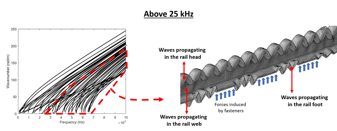
You can check out our paper, “Yang, C., Kaynardag, K. & Salamone, S. Investigation of wave propagation and attenuation in periodic supported rails using wave finite element method. Acta Mech 235, 1453–1469 (2024). https://doi.org/10.1007/s00707-023-03484-8”, where we managed to model the propagation zones of rails across a wide range of frequencies. (To our knowledge, no other study had managed to do this as of the paper's publication date.). You can also check our other papers where we used the waves whose frequencies under 25 kHz to find defect in fasteners, and the waves whose frequencies are over 25 kHz, to find local rail defects.

Case Study: Wave Propagation in Buildings During Earthquakes

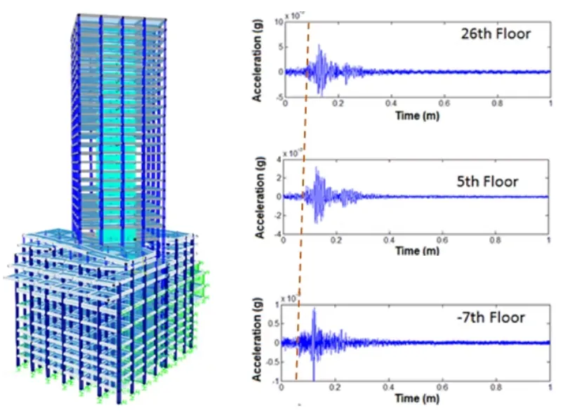
Before wrapping up wave propagation behavior, let me show you the recorded acceleration signals from different stories of a tall building during a small earthquake (Figure 10). I got this figure from my M.Sc. thesis. At the time, I did not notice the time delay in the recorded signals (see the dashed line in the figure, which I added just now); I had no idea, back then, that the earthquake was generating waves that propagated along the structure. There are, in fact, studies that use wave propagation in structures for damage detection, by modeling the structure as continuous or periodic.

Beyond Beams: Plates, Shells, and Pipes

I've been illustrating all of this, the standing waves, the reflections, the mode shapes, using beams as the running example, mostly because a beam's geometry is the simplest one to sketch and reason about. The same underlying logic carries over to other shapes of structure, though: a plate or shell supports waves traveling in two directions instead of one (these are often called Lamb waves), and a pipeline's thin, curved wall guides its own family of wave modes along its length and around its circumference. The bookkeeping gets more involved, with more possible wave modes and more geometry to track, but the physics doesn't change: it's still reflection and interference, and resonance is still just a standing wave that fits the boundaries exactly.

What kind of waves are used in Acoustic Wave Based NDT?

Now let's put everything above to work and talk about the two main families of acoustic wave based nondestructive testing, since this is really the payoff of everything explained in this section. Once you understand how a wave's cross sectional behavior changes with frequency, the logic behind both approaches follows quite naturally, and so does the reason engineers reach for one or the other depending on what they are trying to find.

As I explained earlier, at low frequency a wave's deformation spans the entire cross section, while at higher frequency it becomes shorter in wavelength and can localize in specific parts of the cross section. This same shortening of wavelength is also what makes high frequency waves useful for finding small defects. A wave only reflects strongly off a feature that is comparable in size to, or larger than, its own wavelength; a feature much smaller than the wavelength is essentially invisible to it, in the same way that ocean swell barely notices a small buoy while a short, choppy wave is disturbed by it right away. This is why vibration based SHM, which relies on the low frequency resonance behavior of a whole structure, is good at revealing global condition but cannot pinpoint a small crack, while nondestructive testing deliberately moves up to ultrasonic frequencies, generally taken to be above 20 kHz, where wavelengths shrink down to the millimeter scale or smaller and become sensitive to exactly the kind of small, localized defects that matter for structural integrity.

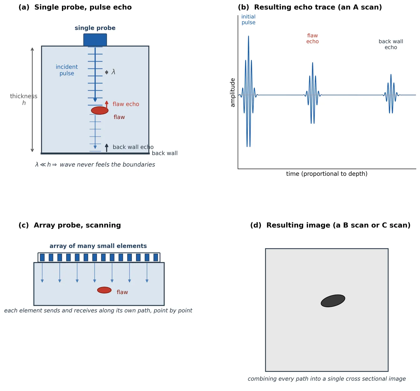
One family is conventional, or bulk wave, ultrasonic testing, shown in Figure 11. A transducer is placed on the surface of the structure and sends a short pulse straight through its thickness. Figure 11 (a) shows this for a single probe: the pulse travels down into the material, and whatever reflects back, an echo from a flaw if one is present, and an echo from the back wall of the part, is recorded by the same transducer and plotted as a function of time. This time trace is called an A scan, shown in Figure 11 (b); because the wave speed in the material is known, the arrival time of each echo can be converted directly into a depth, so a single A scan tells you both whether a flaw is present and roughly how deep it sits. Since the wavelength at these frequencies is so much smaller than the thickness of the part, the wave essentially behaves as it would in an infinite medium: it does not feel the lateral boundaries of the structure at all, and simply travels down, reflects, and comes straight back. This is exactly the high frequency, localized regime described above, just taken to its extreme: the wave is not being guided by the structure's cross section in any meaningful way, it is only bouncing off whatever it hits.

A single probe only tells you about the material directly beneath it, so to inspect a larger area, many probe positions are needed, or, more efficiently, an array of many small elements can be used together, as shown in Figure 11 (c). Each element sends and receives along its own path, and combining every path gives a full, two dimensional image of the region below the array, shown in Figure 11 (d), commonly called a B scan or C scan depending on how the data is presented. This is the imaging mode of ultrasonic testing, and it does not rely on the modal, cross section dependent wave behavior that took up most of this section at all. It is simply using a very short wavelength wave to probe a small region of material directly beneath the probe, point by point, and building up a picture from many such measurements. This makes bulk wave testing extremely good at characterizing a defect once you already know roughly where to look, since it can resolve its size, depth, and shape with good precision. Its limitation is coverage: because each measurement only samples a small local volume, inspecting a long pipeline, a large plate, or an entire rail requires scanning the probe, or the array, over the whole surface, which is slow and, for structures that are hard to access, such as buried pipes or in service rails, often impractical.

The second family is guided wave ultrasonic testing, shown in Figure 12. Instead of sending a wave straight through the thickness, the transducer excites a wave that travels along the length of the structure, using the full cross section as a waveguide, exactly like the waves described throughout the rest of this section on structural dynamics and wave propagation. Because the wave travels along the structure rather than through it, it can reach a defect that is far from the transducer; the wave reflects off the defect and returns to the same transducer as an echo, so a single sensor location can inspect a long stretch of structure, shown schematically in Figure 12 (a), rather than only the small patch of material directly beneath it.

This is where the dispersion curves from earlier in this section become directly useful, rather than just a nice piece of theory. Recall from Figure 4 (a) that a guided wave mode's speed, its phase velocity, generally changes with frequency; a region of the curve where the phase velocity is roughly constant is called non dispersive, and a region where it changes quickly with frequency is called dispersive. What actually governs how fast a wave packet's energy, and therefore its envelope, travels is not the phase velocity but the group velocity, which is the local slope of the dispersion curve. In a non dispersive region, the group velocity stays essentially constant across the narrow band of frequencies contained in a practical tone burst, so every frequency component in the pulse travels at very nearly the same speed, and the pulse arrives at the far end, or returns as an echo, looking much like it started, just delayed and attenuated, as in Figure 12 (c). In a dispersive region, however, different frequency components within the same pulse travel at different group velocities, so the pulse spreads out, or disperses, as it propagates, arriving as a longer, smeared out wave packet that is much harder to time precisely and interpret, as in Figure 12 (d). Figure 12 (b) shows this schematically: the same tone burst launched at two different operating points on two different modes, one flat and one steep, produces a compact echo in one case and a smeared echo in the other. This is exactly why guided wave testing is not simply a matter of picking any convenient frequency: practitioners deliberately choose an operating point, a mode and a frequency, that sits in a flat, non dispersive region of the dispersion curve whenever possible, so that the received signal stays compact and easy to interpret over long propagation distances.

As noted in Figure 12 (a), acoustic emission uses these same guided wave modes, but launches them passively: instead of a transducer sending a pulse, the guided wave is generated by the damage event itself, for example a growing crack or a breaking fiber, and one or more sensors simply listen for it. Everything about how that wave then propagates, its dispersion, its group velocity, its sensitivity to the structure's cross section, is identical to the actively excited case; the only difference is where the wave comes from. Ultrasonic guided wave testing and acoustic emission are, in that sense, the active and passive sides of exactly the same physical phenomenon.

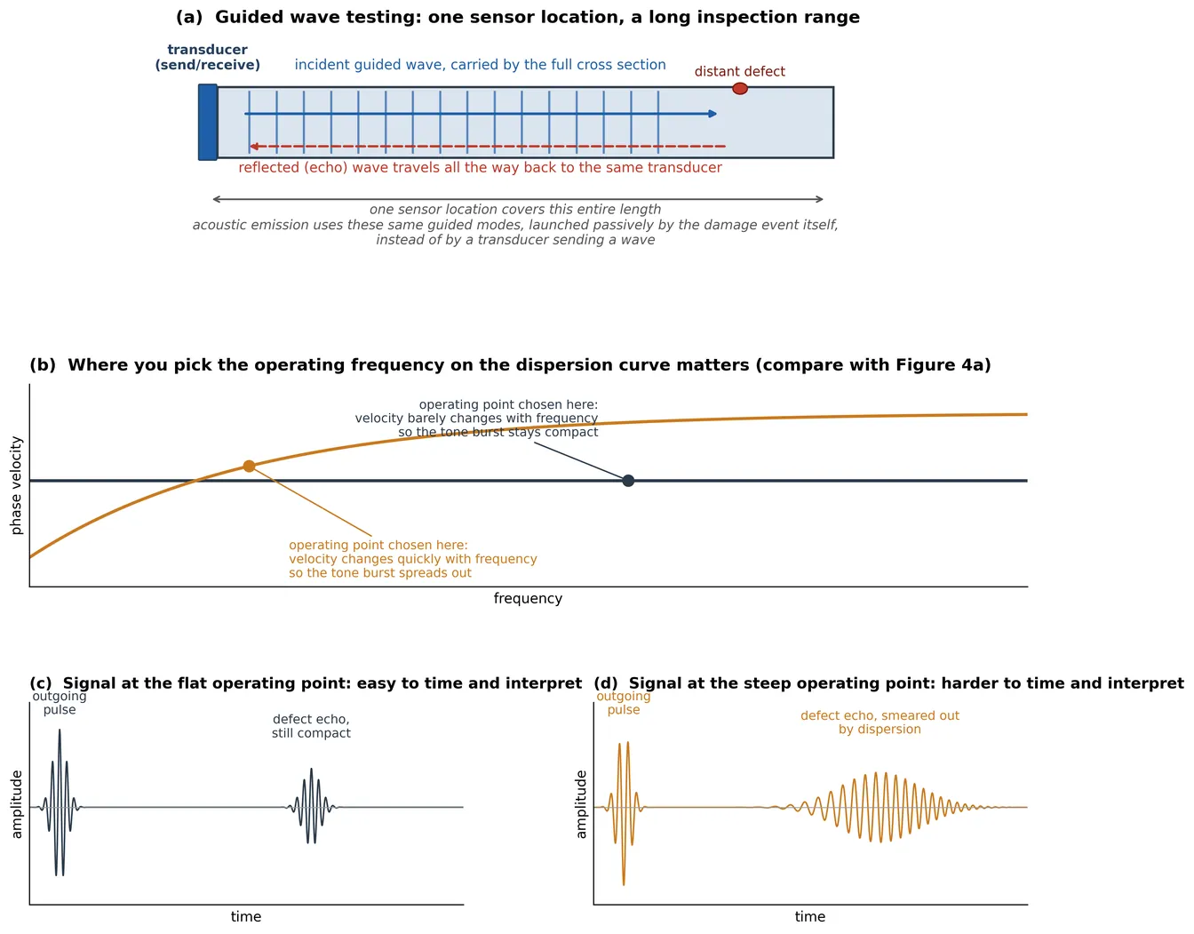
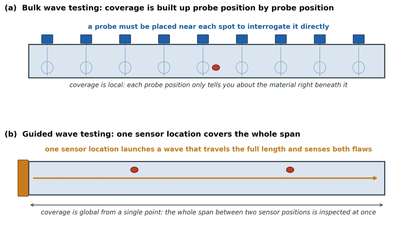
Figure 13 puts the coverage difference between the two families side by side. In bulk wave testing, Figure 13 (a), coverage is built up probe position by probe position, or element by element in an array, and each position only tells you about the material right beneath it. In guided wave testing, Figure 13 (b), a single sensor location launches a wave that travels the full length of the structure and can sense multiple defects along the way, so the whole span between two sensor positions is effectively inspected at once. This is why guided wave testing is so attractive for long, slender structures such as pipelines, rails, and rods, where scanning a bulk wave probe over every inch of surface would be impractical, while bulk wave testing remains the better choice whenever a defect's precise size, depth, and shape need to be characterized once it has already been located.

It is also worth being precise about the term guided wave here, since it gets used a little loosely in my opinion. Guided waves, as a family, are simply the waves that can propagate along a structure, guided by its boundaries; they are exactly the same waves that, depending on the structure's boundary and support conditions and its length, produce resonance frequencies for a finite structure or propagation zones for a periodic or infinite one. In that sense, in my opinion, guided waves are the natural waves that occur in a structure whenever they are exciting, whether by wind, an earthquake, an impact, or anything else; every example of wave propagation in rails shown earlier in this section is a guided wave. Guided waves are not, therefore, inherently ultrasonic: they exist starting from 0 Hz. What guided wave ultrasonic testing does is use guided waves specifically at ultrasonic frequencies, where their wavelength becomes short enough to reflect from small defects like cracks. So guided waves can certainly be used for ultrasonic damage detection, but, again in my opinion, they only become ultrasonic waves once they are used at those higher frequencies; the term guided wave itself does not imply a frequency range.

Table 1 summarizes the practical differences between the two approaches, to make them easier to compare at a glance.

To sum up: every vibration in a structure is, at its root, a wave, and the higher frequency waves are the ones used in nondestructive testing, because their short wavelengths, and their tendency to localize in specific parts of the cross section, make them sensitive to very small defects. Bulk wave ultrasonic testing exploits the high frequency limit where the wave no longer feels the structure's boundaries at all, trading coverage for precision. Guided wave ultrasonic testing instead exploits the same modal, cross section dependent behavior that produces resonance frequencies and propagation zones, just pushed up to ultrasonic frequencies, trading some precision for the ability to inspect a long structure from a single sensor location. Both fall under the active branch of acoustic wave based nondestructive testing, called ultrasonic testing, since an external excitation is deliberately created. The passive branch is called acoustic emission, where instead of creating a wave, we record the transient elastic waves that a structure emits naturally, for example when a crack grows or a fiber breaks. I cover acoustic emissions in more detail in the structural health monitoring and nondestructive testing part of my Research section.

Closing Thoughts

My Ph.D. research was about defect detection in rails, and it was this research that really helped me understand everything I have mentioned in this section. It was difficult at first, since I came from a structural dynamics background, and research articles about rails tended to focus either on wave propagation or on structural dynamics, since rail behaves so differently across different frequency ranges. It took me a while to reach this “aha” moment and put everything together. To my knowledge, I still have not found a brief document that explains: (i) how structures behave at different frequencies in terms of wave propagation, (ii) when resonance frequencies do or do not occur, (iii) when the structural dynamics and wave propagation approaches need to be combined, as with periodic structures, and (iv) what kinds of waves are used in nondestructive testing. That is why I wanted to write this section, to help you see the big picture before diving into structural dynamics and wave propagation. I hope you enjoy reading it.

Recommended Books

• For learning structural dynamics, reading Chopra's well known book, “Dynamics of Structures,” is enough, in my opinion.

• If you'd like to go a step further, into the continuous, rather than discretized, treatment of vibrating structures, Rao's “Vibration of Continuous Systems” is an excellent next step, and it also serves as a nice bridge toward the wave propagation topics below.

• For learning wave propagation, since modeling waves is based on analytical methods in most cases, aside from the semi analytical method, a good understanding of elasticity and continuum mechanics, especially the notation used in the formulations, is required before getting into wave propagation itself. The books “Elasticity: Theory, Applications, and Numerics” and “Continuum Mechanics” are very good for building that foundation. From there, “Wave Motion in Elastic Solids” and “Wave Propagation in Elastic Solids” are, in my opinion, very good books for learning wave propagation itself.

• As I mentioned on the home page, when learning wave propagation, it is better to focus on the type of structure you are actually dealing with. Wave propagation books tend to have separate chapters for different applications, and when I was getting into this field, I thought I needed to learn all of them for my research. I later realized that was not the case. For example, if you are working with beams, pipes, plates, or large media (as in seismology), it is better to focus on the wave motion relevant to that specific type of structure. That said, starting with wave motion in strings and beams is not a bad idea, regardless of what type of structure you ultimately work with.

• Lastly, “Ultrasonic Guided Waves in Solid Media” and “Ultrasonic Waves in Solid Media” are very good books for getting into ultrasonic waves and nondestructive testing.

I hope you find the books I have listed useful as you learn wave propagation and structural dynamics.