 Korkut Kaynardag
Machine Learning: The Complete Picture
Machine Learning
The Complete Picture
Dr. Korkut Kaynardag (Claude is used as help in preparation, especially in figure preparation and proof read)
This guide is meant to show you the big picture of machine learning, so it is meant to be read best before you open a textbook, watch a tutorial on a specific model, or start writing code. It has no equations and assumes no prior knowledge. But of course, you can read it at any point in your machine learning journey. The goal is that, by the end of this document, you can answer ten questions confidently, in your own words, and use those answers as a map for everything you learn afterward.
What does machine learning actually do?
Why do so many different models exist?
What is the difference between non-neural-network-based and neural-network-based models?
What is the working logic of each model?
When should you use which model?
How and why do you need to prepare data for many machine learning models?
What do "data science" and "machine learning engineering" each mean in practice?
How do you know whether a trained model is actually good enough to trust?
What should you watch out for before pointing a model at real people?
Where can you go next to learn more?
The information that answers the question above is explained intuitively at first, explained with a diagram for many cases, along with a real-world example, and zero assumed knowledge.
How to use this guide
Read the document step by step, especially if you are just beginning to learn machine learning. It first gives you the big picture, then explains the main model families one by one. Every model has a diagram, and every concept has a real example. Non-neural network models come first because they are usually simpler and easier to interpret; neural networks come later because they build on the same core ideas but are more powerful on raw, unstructured data. After the individual models, Section 9 covers how to honestly evaluate whether a trained model is actually good, and Section 10 covers how to use these tools responsibly once real people are affected, both are just as important as the modeling techniques themselves. Section 12, "How to Learn Machine Learning," is a set of concrete next steps once you finish.
Scope: this guide covers the core supervised, unsupervised, and reinforcement learning ideas, plus the main neural network architectures (multi-layer perception (MLP), convolutional neural networks (CNN), recurrent neural networks (RNN)/Long-short term memory (LSTM), Transformer). It does not currently cover graph-based machine learning (Graph Neural Networks) or generative models (GANs, diffusion models, VAEs) as those are large enough topics that they deserve their own guide, and people usually do not jump into learning them before learning the material/methods in this document.
Why did I prepare this document: when I was learning machine learning, it took me a long time to understand how the different models actually work in simple logic, what the difference between neural-network and non-neural-network methods is, when to use each one, why and how to prepare data, and, most importantly, the complete big picture of machine learning. So, I wanted to prepare this document in case it could be helpful for other interested people.
Disclaimer: everything in this document reflects my own knowledge and experience. If anything here contradicts your own knowledge or experience, please reach out so it can be fixed: korkutkaynardag@iyte.edu.tr
1. What is Machine Learning?
Classic programming means you write the rules. For example: "If a transaction is over $10,000 and happens at 3am, flag it as suspicious." Machine learning is different: instead of writing the rules, you show a program thousands of labeled examples and let it figure out the rules itself.
That is it. ML is finding patterns in data so that you do not have to write the rules by hand. Every model, for example, Support Vector Machines (SVMs), decision trees, neural networks, and everything in between, is just a different strategy for doing that learning. (SVMs and decision trees are non-neural network models, as the table below explains.)
Underneath the variety, every model in this guide learns in the same basic way, and it is worth having that idea before the individual models start. A model is a function with adjustable numbers inside it, called parameters: the weights in a linear regression, the split thresholds in a decision tree, the millions of weights in a neural network. Training means choosing those numbers. You define an objective, which is a measure of how wrong the model's current predictions are on the training data, and then you search for parameter values that make that measure small. Sometimes the best values can be solved for directly, as in linear regression; sometimes they are chosen greedily one step at a time, as a decision tree picks its splits; and sometimes they are nudged a little at a time over many passes through the data, which is what gradient descent does in a neural network (Section 5.3). When training stops, the parameters are frozen and the model is applied to new inputs it has never seen. Models differ in what their parameters represent and how that search is carried out. They do not differ in that basic pattern, and it is the reason Section 9 exists: scoring well on the data you fitted is easy, while scoring well on inputs you have not seen is the actual goal.
There are two major families of ML models, and understanding the difference between them is the single most useful mental model you can have, as long as you hold it as a practical default rather than a hard boundary. Both families are more flexible than the split below suggests, and Sections 1.2 and 8 come back to exactly where it bends:
Non-Neural Network Models | Neural Network Models |
|---|---|
These models usually learn from meaningful features that a human has prepared such as age, income, transaction count, lab values. They are often fast, interpretable, and very strong on structured or tabular data. You decide what the model sees. Typical tasks: classification, regression, clustering, anomaly detection, and forecasting on structured data. Typical domains: healthcare, finance, retail, manufacturing, insurance, sports analytics, and any domain with well-organized tables or databases. | These models can solve the same prediction tasks, but they especially shine when the input is raw or unstructured such as images, audio, text, video, or complex sensor streams. The network learns useful internal features through its own layers. The model learns what to look at. Typical tasks: classification, regression, forecasting, language modeling, image understanding, audio processing, and representation learning. Typical domains: computer vision, speech, language AI, robotics, medical imaging, recommendation systems, and large-scale applications where automatic feature learning helps. |
The key insight to table above! Both model families can perform many of the same tasks. The main difference is not the task itself, but the form of data each family handles most naturally, and how much of the feature work is done by the human versus the model. Non-neural network models: strongest on structured tables with meaningful, human-prepared features such as age, income, lab values, transaction counts, sensor summaries, or text vectors. Neural networks: strongest on raw or unstructured data: images, sound, text, video, complex sensor streams, because they can learn useful internal features through their layers. Practical boundary: this is a useful default, considering today’s machine learning practices, but not a strict rule. Non-neural models can work with images, audio, or text after feature extraction (which, I am sure, you will see some examples when you learn ML in deep), and neural networks can work with structured tables, though neural networks are usually most valuable when automatic feature learning gives a clear advantage. Thus, we can use Figure 1 to demonstrate non-neural network and neural network models’ use cases. Simple way to remember it: with non-neural network models, you usually decide what the model sees. With neural networks, the model often learns what to look for. | |
All machine learning models, whether neural or non-neural, are built around this same small set of core mechanisms. Figure 2 presents them not as separate topics to study one by one, but as the basic patterns behind every application in this guide, including the image, audio, and NLP problems in Section 6. Recognizing a cat in a photo, marking an email as spam, and flagging a tumor in an X-ray are all classification tasks because only the raw input changes: pixels, words, then pixels again. Predicting tomorrow's demand is forecasting; predicting a house price is regression; grouping similar customers or documents is clustering. Whenever a later section introduces a model for images, audio, or text, it is worth asking which of these five mechanisms it is using. The answer is always one of them, applied to a different kind of raw input, but in different ways.
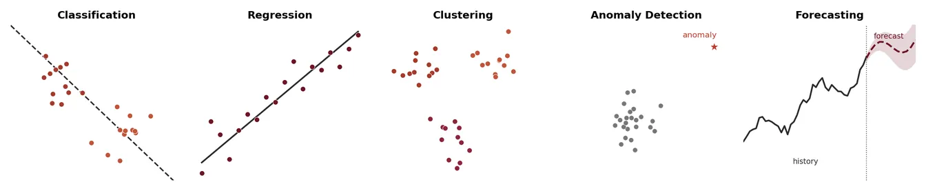
That being said, Section 4, which explains non-neural ML methods, makes these mechanisms easy to see directly in math and the diagrams. The neural network sections (5 and 6) often hide them behind layers of neurons, but underneath, a neural network is still doing one of these same five things: fitting a separating surface, fitting a regression function, discovering structure, or estimating future values. It is just doing it with a much more flexible, layered function. In that sense, a neural network can be described as a "tuned, complex function approximator." Section 12, "How to Learn Machine Learning," points to video resources including the StatQuest YouTube channel's neural network series that make this very visual and concrete; a good starting point there is the playfully titled video on YouTube: StatQuest Happy Halloween (Neural Networks Are Not Scary).
1.1 Supervised vs. Unsupervised: Not Every Task Needs Labels
Figure 2 groups five task mechanisms together, but they actually split into two very different setups depending on whether you have labels at all, and both families of models from the table above show up on both sides of that split.
Classification and regression are supervised learning tasks: these names describe what the model is trying to predict, not which type of model must be used. In both cases, the training data includes examples where the correct answer is already known. A classification task predicts a category such as approved or declined, spam or not spam, tumor or not tumor. A regression task predicts a number such as a house price, a patient risk score, next month's demand. Either model family can learn these tasks: a non-neural model such as logistic regression, a decision tree, or a Random Forest usually learns from features a human has prepared, while a neural network such as a Multilayer Perceptron (MLP), a Convolutional Neural Network (CNN), or a Transformer can solve the exact same kind of task but often learns useful features directly from raw pixels, audio, or text. So supervised learning defines the goal; the model family only defines how the input is represented and learned.
Forecasting is supervised learning too: a special case of regression: The "label" is simply the value at a future point in time, learned from a history of past values. Non-neural models handle it with methods like ARIMA (a classical statistical model that predicts the next value from a weighted combination of recent past values and past errors), exponential smoothing, or gradient-boosted trees trained on lagged features (an ensemble-of-trees method explained in Section 8); neural networks handle it with sequence models such as Recurrent Neural Networks (RNNs), Long Short-Term Memory networks (LSTMs), and Transformers that read the historical sequence directly (Section 6). Either way it still needs a labeled history to learn from, which is why it belongs on the supervised side with classification and regression rather than with clustering.
Clustering is unsupervised learning: There is no known answer to learn from at all, only unlabeled data, and the model's job is to discover structure in it on its own. For example, grouping customers into segments nobody had pre-defined (Section 4.8). Non-neural models are not limited to supervised tasks: K-Means is a non-neural model that works with zero labels, which is exactly why it belongs in the same family as linear regression and decision trees even though it never sees a "correct answer." Neural networks have unsupervised methods of their own: an autoencoder is a neural network trained only to compress and reconstruct its own input, with no labels anywhere in that process, and the compressed representation it learns can then be clustered. So clustering, like classification and regression, is not the exclusive property of either family. It is the presence or absence of labels that defines it, not which family is doing the work.
Anomaly detection can go either way: Most often it is unsupervised too. The model learns what "normal" data looks like on its own and flags anything that does not fit, with no labeled examples of past anomalies required, though a supervised version is possible when labeled examples of known anomalies already exist. The neural version of the unsupervised case is usually built on that same autoencoder idea: trained only on normal data, it learns to reconstruct normal examples well and anomalies poorly, and that reconstruction error becomes the anomaly score (equivalent of a non-neural distance) or density-based method (Section 4) that learns the shape of "normal" with no labeled anomalies at all.
This distinction matters in practice: unsupervised methods let you get started on a dataset that has never been labeled at all, which is often the more realistic starting point, while supervised methods require that someone has already labeled a reasonable number of examples by hand first. Section 7 introduces a third setup, reinforcement learning, which needs neither labels nor pre-existing structure since it learns from the consequences of actions instead.
1.2 Why Non-Neural Models Are Considered “Simpler”
Calling non-neural network models "simpler" is not just a figure of speech; it is true in two very concrete ways: what they are able to do on their own, and how much computation they cost.
What they can do on their own: A non-neural model has no built-in way to make sense of raw pixels, raw audio samples, or raw text. The math for these algorithms, such as a weighted sum in linear or logistic regression, a yes/no split in a tree, a distance calculation in K-Nearest Neighbors (KNN), assumes each input number is already a meaningful, self-contained piece of information, such as an age, a credit score, or a pixel count above a threshold. It has no mechanism, like a CNN's convolutional filters or a Transformer's attention, for discovering that a group of neighboring pixels forms an edge, or that a stretch of audio samples forms a rising pitch. That discovery step has to be done by a human first (feature engineering, Section 3.4). A neural network, by contrast, can be hierarchical and learn that structure itself directly from the raw signal. So it is not that non-neural models are mathematically incapable of unstructured data. It is that they depend on you to do the hard part of understanding the raw signal before they ever see it.
Computational load: Non-neural models are also simpler in the literal sense of requiring far less computation. A logistic regression or a decision tree might have anywhere from a handful to a few thousand parameters, trains on a laptop CPU in seconds to minutes, and needs only a modest amount of labeled data to fit well. A neural network doing the same job on raw data typically has hundreds of thousands to billions of parameters, is fit through many iterations of gradient descent and backpropagation (Section 5.3 explains these), and in most practical cases needs a GPU (a graphics processing unit which is a chip originally built for rendering images, but very good at the kind of parallel math neural networks need) and a large, labeled dataset to train in a reasonable amount of time. At inference (prediction) time the gap remains: a decision tree walks a handful of yes/no questions, while a deep neural network runs millions of multiplications per prediction. This is why non-neural models are still the default choice for structured data and for any setting with tight compute, memory, latency, or power budgets. For example, a fraud-detection rule that must score a transaction in milliseconds on a CPU, or a model running on a small embedded device (I will not talk about running ML models in small micro-chips like the ones in your smart home devices and air conditioners, and even in your toothbrush nowadays, but you can usually run only small non-neural network models or very small neural network based models on those microchips, which is called edge AI; In general, bigger models run on cloud or on strong hardware).
It works in the other direction too: Neural networks are not restricted to unstructured data. A plain MLP (Section 5.2) can take the exact same tabular feature vector as a logistic regression or a Random Forest and produce the exact same kind of classification or regression prediction. Structured, tabular problems are usually not solved with neural networks not because they cannot do the job, but because the extra computational cost rarely buys any extra accuracy there: on tabular data, a well-tuned Random Forest or XGBoost model (a popular gradient-boosted-tree method, explained in Section 8) typically matches or beats a neural network anyway, for a fraction of the training time. Neural networks earn their keep specifically on unstructured data, where non-neural models are capability-limited as described above, rather than simply outperformed. Read all of this as a statement about what usually happens, not about what is possible. Gradient boosting is not inherently weaker than a neural network, and a neural network is not inherently weaker on a table. Which one wins on a given problem depends on how much data you have, how the features are represented, how noisy the data is, and how much compute and tuning time you can spend, so for any specific dataset the honest answer is to try both and compare properly (Section 9).
Data science vs. machine learning engineering
Data science and machine learning engineering overlap, but they usually emphasize different parts of the workflow. Data science normally starts with a dataset and a question. Machine learning engineering is more focused on building, training, deploying, and maintaining ML systems, especially when the input is large, raw, unstructured, or continuously changing.
Data science usually works with datasets: structured or semi-structured data where each row is an example and each column is a feature. Examples include patient records, customer purchases, loan applications, demand history, lab results, survey answers, sensor summaries, transaction logs, and website activity.
Data science tasks: understand the problem, clean and join data, explore patterns, create features, visualize results, build statistical or ML models, evaluate errors, explain findings, and support decisions. Typical tasks include classification, regression, forecasting, clustering, anomaly detection, segmentation, reporting, and decision support.
Data science models: statistical analysis, visualization, data mining, linear regression, logistic regression, decision trees, Random Forests, Support Vector Machines, K-Nearest Neighbors, K-Means, and sometimes neural networks when they add value.
Machine learning engineering often works with raw or large-scale data: images, audio, video, text, documents, speech, sensor streams, robot camera feeds, clickstreams, recommendation logs, and very large training datasets. These are still data, but the challenge is usually building a system that can learn useful representations and run reliably in production.
Machine learning engineering tasks: design training pipelines, prepare large datasets, train and tune models, manage GPUs and compute, deploy models, serve predictions, monitor performance, retrain models, handle data drift, and integrate the model into an application or product.
Machine learning engineering models: neural networks are common when the data is raw or unstructured, such as Convolutional Neural Networks for images, Transformers for text and large language models, Recurrent Neural Networks and Long Short-Term Memory networks for sequences, and specialized models for speech, robotics, recommendation, and computer vision.
Important overlap: this is not a strict boundary. Data scientists may build neural networks, and machine learning engineers may use non-neural network models. The difference is usually the emphasis. Data science focuses more on extracting insight from datasets. Machine learning engineering focuses more on turning ML models into reliable systems.
Simple way to remember it: data science asks, “What can this dataset tell us?” Machine learning engineering asks, “How do we build a working ML system that learns from data and keeps working in the real world?”, but again also remember, both can have the tasks mentioned above in each other’s categories above.
2. More Usage Examples, by Domain
Section 1 explained the main idea: both non-neural network models and neural networks can solve many of the same ML tasks, but they are usually most useful in different situations. This section gives more usage examples across real domains so you can see the practical pattern repeat. Non-neural models are usually the first choice for structured datasets such as tables of patients, transactions, customers, machines, or products. Neural networks are usually preferred when the data is raw, unstructured, very large, or naturally sequential: images, audio, text, video, speech, robot sensor streams, or large recommendation logs.
Domain | Non-Neural Model Use Cases | Neural Network Use Cases |
|---|---|---|
Healthcare | • Readmission risk from patient records • Drug dosage regression from lab values • Disease risk scoring from structured history • Patient clustering from age, diagnosis, labs • Hospital length-of-stay prediction | • X-ray, MRI, and CT image diagnosis • Medical image segmentation (tumors, organs) • Clinical note summarization and coding • ECG and medical signal anomaly detection • Voice analysis for speech or neurological disorders |
Finance | • Fraud detection from transaction features • Credit scoring from applicant records • Customer churn prediction • Loan default probability estimation • Cash-flow and portfolio-risk forecasting | • Invoice and contract document processing • News and earnings-call sentiment analysis • Identity verification from image or voice • Large-scale fraud pattern learning • Automated customer-support chatbots |
Manufacturing | • Predictive maintenance from sensor summaries • Demand and inventory forecasting • Sensor anomaly detection • Process quality classification • Reject-rate prediction from machine settings | • Visual defect detection from camera images • Audio-based machine fault detection • Robot navigation from camera feeds • Real-time visual inspection systems • Digital-twin sensor sequence modeling |
Retail / E-commerce | • Churn and lifetime-value prediction • Price elasticity regression • Customer segmentation • Demand forecasting from sales history • Basket analysis and product affinity | • Visual product search • Product image classification • Review sentiment and product-text analysis • Personalized recommendation systems • Search ranking from click and text signals |
Education | • Student dropout-risk prediction • Grade prediction from attendance and scores • Student grouping by learning behavior • Course demand forecasting • At-risk course or program detection | • Automated essay feedback • Lecture transcription and summarization • Personalized tutoring chatbots • Handwriting and diagram recognition • Speech-based pronunciation feedback |
Transportation | • Delivery-time prediction from route features • Traffic demand forecasting • Fleet maintenance risk scoring • Route-delay classification • Driver risk scoring from trip summaries | • Self-driving perception from cameras/lidar • Driver behavior recognition from video • Speech interfaces in vehicles • Scene understanding for navigation • Road sign and lane detection |
Cybersecurity | • Login anomaly detection from access logs • Phishing risk scoring from email metadata • Network intrusion classification • User behavior clustering • Alert prioritization from incident records | • Malware classification from code patterns • Phishing detection from email text and links • Threat report summarization • Sequence modeling of attack behavior • Automated incident report generation |
Agriculture | • Crop yield prediction from weather/soil data • Irrigation-need classification • Pest risk forecasting from field records • Farm-zone clustering from sensor summaries • Fertilizer recommendation from soil features | • Crop disease detection from leaf images • Drone image field monitoring • Livestock behavior recognition from video • Weed detection for autonomous spraying • Animal sound monitoring for health alerts |
Noting again: every use case in the left-hand column is a classification or regression task, and neural networks are just as capable of all of them. A neural network can score fraud, predict churn, or estimate readmission risk exactly like the non-neural models listed there do. This table places each use case under whichever family is the practical default today (Section 1.2): non-neural models when the data is structured and tabular, neural networks when the data is raw and unstructured, or when the dataset is large enough that learning the features automatically pays off.
3. Features, Preprocessing, and Feature Engineering
Every machine learning model ultimately receives numbers. A feature is one input value that describes one aspect of an example such as age, income, temperature, word count, average vibration. The complete set of features for one example is a feature vector. Many examples together form a feature matrix, similar to a spreadsheet where each row is one example and each column is one feature. This section explains the full path from messy raw data to a clean feature matrix a model can learn from.
The clean workflow
Keep these steps separate in your mind → explore the data, clean the data, engineer useful features, select the most useful features, then train the model. Data exploration helps you understand what is inside the dataset. Preprocessing fixes practical problems such as missing values, inconsistent formats, and different scales. Feature engineering creates better inputs from domain knowledge. Feature selection removes weak or risky inputs. Neural networks still need clean input, but they can often learn useful internal features from raw or lightly processed data.
3.1 From Raw Data to a Feature Matrix
The goal of Section 3 is to explain how raw information becomes model input. Raw data may be a spreadsheet, a database table, a transaction log, a sensor stream, a document, an image, or an audio file. Before a model can use it, the useful parts must be represented as numbers. In a typical tabular dataset, each row becomes one example and each column becomes one feature. For non-neural network models, this feature matrix is especially important because the model usually depends on the human to decide what information should be visible. Figure 3 summarizes the full pipeline visually, from raw data to a ready feature vector.
A useful pipeline is as follows:
Explore: understand distributions, missing values, outliers, correlations, and possible leakage before changing the dataset.
Clean and preprocess: impute/estimate missing values; fix duplicate rows, inconsistent units, invalid entries and inconsistent categories; and train/test leakage risks.
Feature Engineering: extract, transform, encode, and normalize information so the model receives useful numeric inputs.
Select features: keep useful inputs and remove features that are irrelevant, redundant, noisy, leaking the answer, or too expensive to collect.
Raw Data | Explore | Clean | Feature Engineering | Select | Feature Vector |
|---|---|---|---|---|---|
records, logs, images, audio, text | missingness, outliers, imbalance, leakage | impute, standardize, balance, fix units | extract, transform, encode, normalize | remove weak, duplicate, leaking features | numbers ready for a model |
3.2 Data Exploration (another name: Data Mining)
Exploration Question | What You Check | Why It Matters |
|---|---|---|
Are values distributed normally? | Histograms, skewness, extreme values | Shows whether log, power, or binning transforms may help. |
Are values missing? | Missing-value rate and pattern | Shows whether imputation is safe, and whether missingness itself should become a feature. |
Are features redundant? | Correlation analysis, duplicate/near-duplicate columns | Highly similar inputs can make the model harder to interpret and less stable. |
Is the target leaking? | Columns created after the event, future information, direct proxies for the answer | Leakage gives fake accuracy during training and fails in real use. |
Are classes imbalanced? | Class counts, rare-event frequency | If found, handle it during preprocessing and evaluation instead of trusting accuracy alone. |
3.3 Data Cleaning
After exploration, the next step is to make the dataset reliable. Cleaning and preprocessing fix practical problems that would otherwise confuse the model or create misleading results. This step does not try to invent new meaning yet; it makes sure the data is consistent, usable, and safe to train on.
Common cleaning and preprocessing steps:
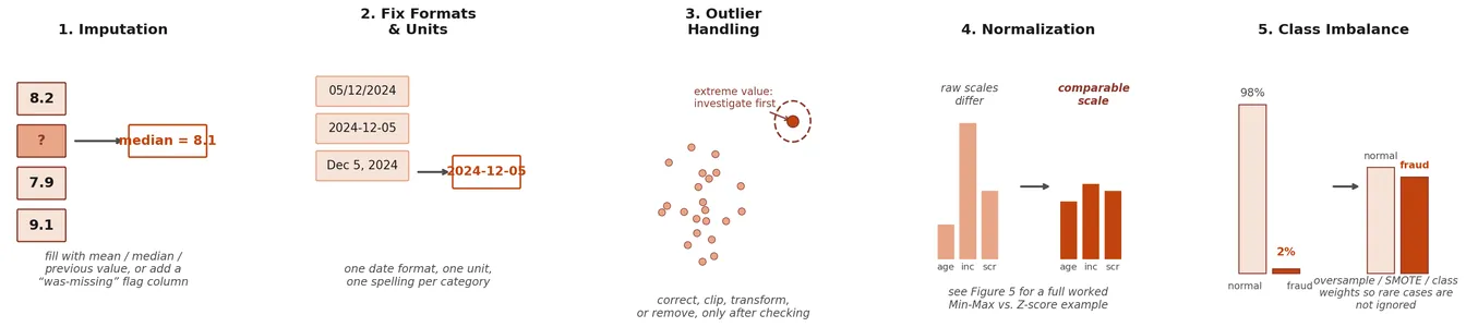
Imputation: Fill missing values with a reasonable estimate such as the mean, median, mode, a previous value in a time series, or a model-based estimate. Sometimes the fact that a value was missing is itself useful, so a missing-value indicator column can also be added. More complex methods exist too, such as K-nearest-neighbors imputation, which fills a value using the average of the most similar rows, or regression imputation, which predicts the missing value from the other columns with a small trained model. Other methods exist as well, which can be mostly adopted from missing value estimation studies in the literature. Or, develop your own 😊. Remember, there will be trade-off between each imputation approach that you will select.
Inconsistent formats and units: Make values comparable before modeling. Dates should use one format, categories one spelling, measurements one unit. For example, height should not be mixed between centimeters and inches unless it is converted first.
Outlier handling: Investigate extreme values before deciding what to do. Some outliers are real and important, such as a very large fraud transaction; others are data-entry mistakes. Possible fixes include correcting, clipping, transforming, or removing them.
Normalization and standardization: Rescale numeric features so they are comparable. Important for distance-based models, SVMs, gradient descent, and neural networks. Less important for decision trees and Random Forests, which split on feature thresholds rather than distances. Figure 5 compares Min-Max scaling and Z-score standardization side by side on the same three features.
Class imbalance handling: Fix cases where one class is much more common than another, such as 98% normal transactions and 2% fraud, otherwise a model can look accurate by predicting the majority class almost every time. Common fixes: stratified train/test splitting (keeping the same class balance in both splits), oversampling the minority class, under sampling the majority class, synthetic minority examples (SMOTE, which generates new synthetic examples of the rare class instead of just duplicating existing ones), class weights (telling the model that a mistake on the rare class costs more during training), threshold tuning (moving the decision cutoff away from the default 0.5), and metrics such as precision, recall, F1, ROC AUC, and PR AUC (all defined in the Glossary, Section 11, and explained with a confusion matrix in Section 9.4). For rare event problems like fraud, disease detection, equipment failure, or security alerts, recall and precision are usually more informative than accuracy.
Figure 4 below walks through all five of these steps on a small worked example.
Before Scaling | Min-Max Scaling | Z-Score Standardization |
|---|---|---|
age = 42 income = 87,000 credit_score = 742 | age = 0.47 income = 0.34 credit_score = 0.61 | age = −0.21 income = −0.22 credit_score = +0.18 |
3.4 Feature Engineering for Non-Neural Models
Feature engineering is where domain knowledge becomes model input. This step creates useful columns from raw records, and it matters especially for non-neural network models: these models usually do not discover hidden structure directly from raw pixels, audio, or text on their own. They perform best when a human prepares meaningful features first.
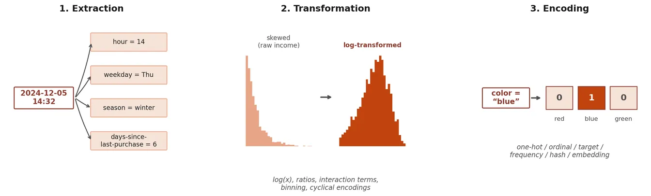
Extraction: Pull useful information out of raw fields. A timestamp can become hour, weekday, weekend flag, season, or days-since-last-purchase. A transaction history can become average order value, purchase frequency, return rate, or spending change over time.
Transformation: Change the scale, shape, or meaning of a feature so patterns become easier to learn such as log transforms for skewed money values, ratios like debt-to-income, interaction terms like age × risk score, binning into low/medium/high, cyclical encodings for hour or month.
Encoding: Convert non-numeric information into numbers. Common techniques: one hot encoding, ordinal encoding, label encoding, binary encoding, frequency encoding, count encoding, target encoding, hash encoding, bag of words, term frequency inverse document frequency, embeddings, date encoding, cyclical sine and cosine encoding, and missing value indicator encoding.
For example, in a hospital readmission model, useful features might include age, previous admission count, diagnosis group, lab ratios, medication count, and length of stay. Weak or risky features might include patient ID, duplicate lab columns, columns missing for most patients, or a discharge code that indirectly reveals the answer.
Figure 6 below walks through all three of these steps on a small worked example.
3.5 Feature Selection and Dimensionality Reduction
After features are created, the final feature set should be simplified: more columns are not always better. Irrelevant, duplicated, noisy, expensive, or leaking features can make the model slower, harder to interpret, and more likely to fail on new data. Feature selection keeps only the inputs that genuinely help prediction.
Filter methods: Score features before training, using correlation, variance, chi-square tests (a statistical test for whether a feature and the target are related), mutual information (how much knowing one variable reduces your uncertainty about another), missing-value rate, or duplicate checks. Fast and useful for early cleanup.
Wrapper methods: Train the model repeatedly with different feature subsets and keep whichever performs best: forward selection, backward elimination, recursive feature elimination. Effective but can be slow.
Embedded methods (some models can inherently do this task): let the model identify important features during training itself such as L1 regularization (a training penalty that pushes unhelpful feature weights toward exactly zero, effectively removing them), decision tree splits, Random Forest or gradient-boosted-tree feature importance.
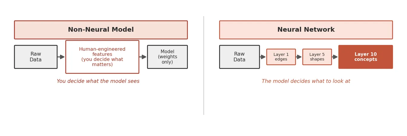
Dimensionality reduction: create a smaller set of new features that summarize many original ones. Principal Component Analysis (PCA) is the classic example. It is useful when many features are correlated or noisy, though the new components can be harder to explain than the original columns. Figure 7 contrasts this human-driven feature engineering with the feature learning neural networks perform automatically, covered next in Section 3.6.
Neural networks still benefit from preprocessing Even though neural networks learn their own features, you still need to: normalize pixel values (0-255 to 0-1), handle missing values, ensure data is in the right format, and often apply data augmentation (random flips, crops, noise) to help the network generalize. The difference is you are not deciding what features matter, you are just cleaning and standardizing the raw input. | |
Feature Engineering | Feature Learning |
Human creates features first such as ratios, counts, bins, text vectors, image descriptors. Non-neural models use these directly. | Model learns internal features such as edges, textures, sound patterns, word context. Neural networks learn these through layers. |
3.6 Feature Learning in Neural Networks
In images, early layers may learn edges and textures, while later layers learn object parts and larger visual patterns. In audio, a waveform or spectrogram lets the network learn sound patterns over time. In text, embeddings and attention let the network learn meaning from word context. This is why neural networks are so useful for raw or unstructured data such as images, audio, video, language, and robotics.
Neural networks still need clean and correctly formatted input, but they often reduce the need for hand-designed features. Instead of giving the model explicit features such as edge count, average pitch, or word frequency, you provide raw or lightly processed input and let the network learn useful internal representations through its own layers.
A quick caveat on "raw.": "Raw data" does not always mean the data arrives completely untouched. Audio is the clearest example: as Section 6.2 covers in detail, the raw waveform is normally converted to a frequency-domain view (a spectrogram) before a CNN ever sees it, because that view lays out sound's structure in a way convolutional filters can use far more efficiently. That conversion is still "raw" in this guide's sense, because it reorganizes the signal rather than deciding what matters inside it. It is not a choice-free step, though: window length, overlap, and frequency resolution are real decisions, and they trade detail in time against detail in frequency, so a spectrogram is not a perfectly lossless view of the waveform either. The distinction that matters here is that those choices set how the sound is displayed, not which patterns count as meaningful. The network still has to discover which patterns in it are meaningful, the same as with untouched pixels. Section 6.2 explains why this is not the same thing as the hand-engineered feature extraction described in Section 3.4.
Accordingly, in my experience and in general practice, 50 to 80% of the coding/tasks about data preparation, especially for non-neural networks, 10-30% model generation, 10-30% result reporting.
4. Non-Neural Network Models
These models are the backbone of real-world ML in business, healthcare, and science and similar domains. They are usually fast, often easy to interpret, and excellent when the data is structured. Interpretability deserves one caveat, because it varies a great deal inside this family rather than being a property all of them share: a linear model or a small decision tree can be read directly, one line at a time, while a Random Forest of hundreds of trees, a boosted ensemble, or a kernel SVM is much harder to read and usually needs dedicated explanation tools such as feature-importance scores or SHAP values before an individual prediction makes sense. Doctors, banks, and insurance companies often prefer the simpler end of this family for exactly that reason, because you can explain every single prediction. As mentioned before, they can be also used for images, audio, text analysis as well. I will not go into mathematical details as this document’s scope is to give the big picture of machine learning.
4.1 Linear Regression: Predict a Number
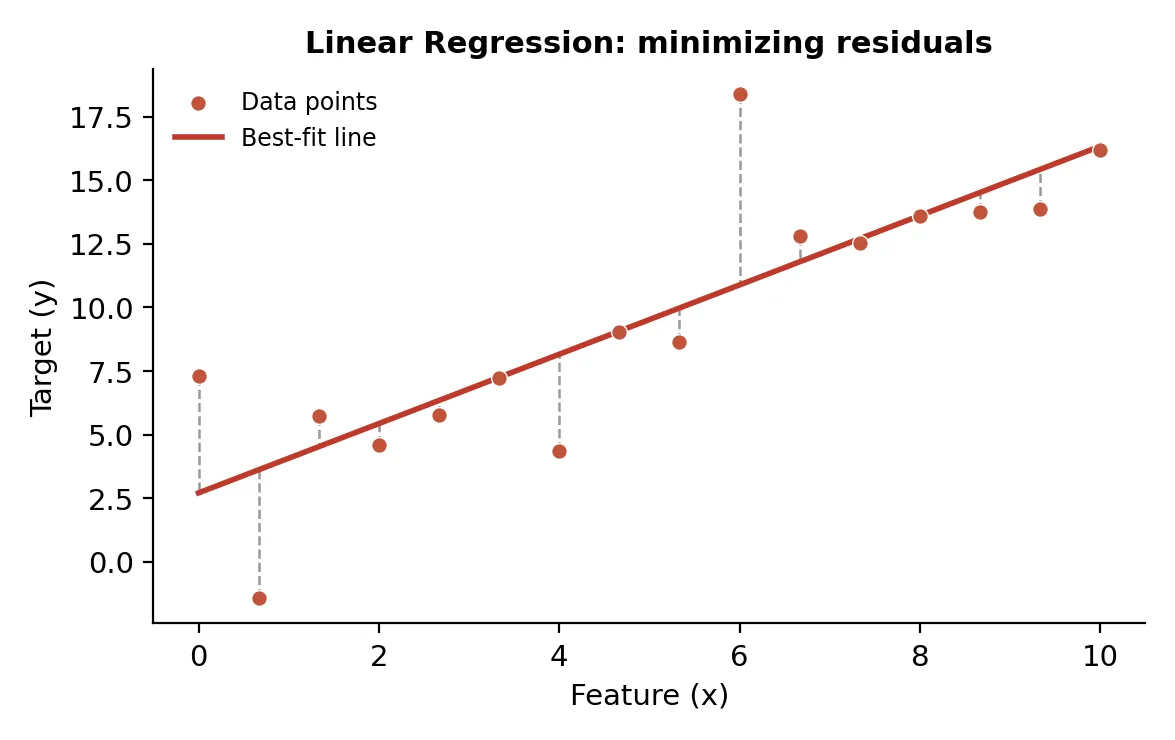
Finds the best-fit line (or hyperplane which is the same idea as a line, just in a space with more than one input feature) through your data. Prediction is simply the weighted sum of features: each feature is multiplied by its own learned weight, a number that captures how strongly that feature moves the prediction, and a bias term is added on top. For example, a house price might be predicted as (weight1 × square footage) + (weight2 × number of bedrooms) + bias. The model learns the specific weight values that minimize prediction error. Works for any continuous output, is simple and fast, and is a natural baseline before trying more complex models. It works best when the relationship is reasonably linear and the data is not dominated by extreme outliers. Figure 8 shows what "best fit" means in practice: the line is positioned to minimize the total squared distance between itself and every data point.
Real-world: hospital readmission risk score, product demand forecasting, drug dosage response, house price estimation, insurance claim amounts
Use it when: the target is a number, the relationship is close to linear, and you want a fast, fully explainable baseline before trying anything more complex because the weight of features demonstrate how much each feature has an effect on the outcome.
Think twice when: the pattern is strongly nonlinear, the features interact heavily in ways you have not built in by hand, or a few extreme outliers dominate the fit.
4.2 Logistic Regression: Yes/No Decision with a Probability
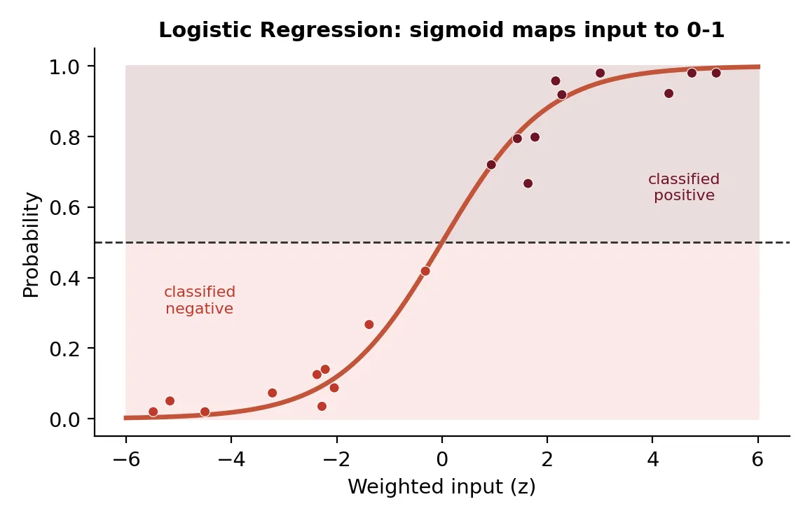
Used for classification, even though its name contains the word regression. It calculates a score from the input features, then converts that score into a probability between 0 and 1. This makes it useful when you need both a decision and a confidence level, such as a probability of readmission or fraud. The decision threshold can be adjusted depending on the problem: instead of always using 0.5, a Receiver Operating Characteristic (ROC) curve plots the true positive rate against the false positive rate at every possible threshold, so you can see exactly what is gained and lost by moving the cutoff up or down, and choose the threshold that fits what a mistake actually costs (Section 9.4 explains ROC curves and the confusion matrix behind them in full). For example, in case of disease screening, you may prefer to catch more possible cases, even if that creates more false alarms. Figure 9 shows the S-shaped sigmoid curve that produces this probability, with the default 0.5 threshold marking where a prediction flips from negative to positive.
Real-world: tumor malignant/benign, email spam/not-spam, loan approve/decline, patient readmission yes/no
Use it when: you need a yes/no decision together with a probability you can threshold, and you have to be able to explain each prediction to a regulator, a clinician, or a customer.
Think twice when: the real boundary between classes is genuinely curved, or the useful signal lives in feature interactions that you would have to construct manually.
4.3 Decision Tree: A Flowchart of Questions
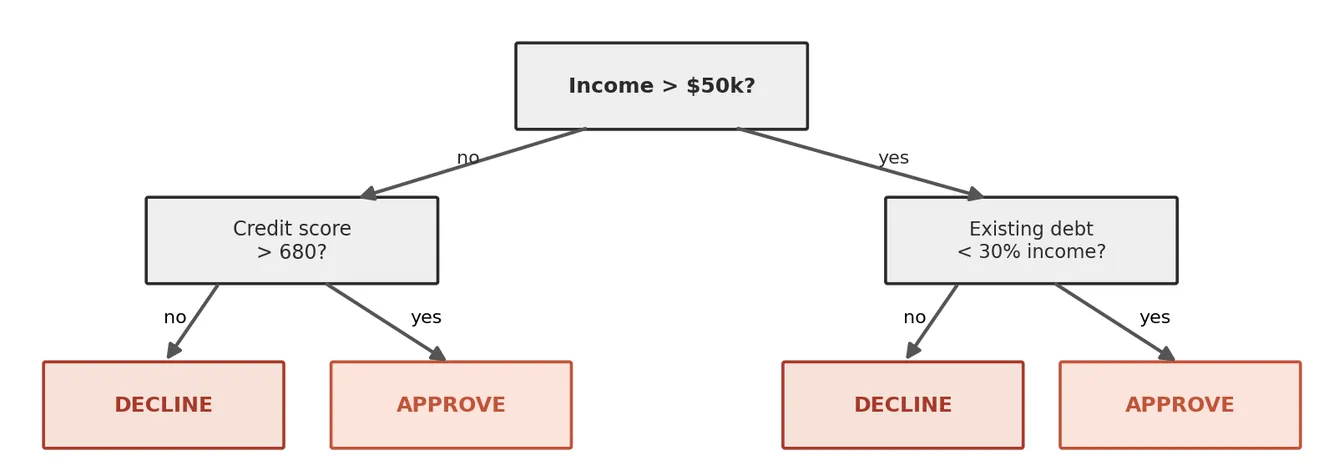
It learns a sequence of yes/no questions through the features. Each split divides the data into smaller groups, and each path ends at a prediction. The model is easy to explain because you can follow the exact route from input to output, which makes it useful wherever transparency matters: healthcare, finance, insurance, policy decisions. A single tree can overfit if it grows too deep, so tree depth and minimum leaf size are important controls. Figure 10 shows a worked example for loan approval: every internal node is a yes/no question, and every leaf is a fully auditable decision.
Real-world: medical diagnosis protocols, credit scoring, fraud rules, insurance underwriting, customer eligibility checks
Use it when: transparency matters more than the last few points of accuracy, and someone needs to follow the exact path from input to decision.
Think twice when: you want the best possible accuracy: a single tree is unstable, since a small change in the data can reshape it entirely, and an ensemble of trees almost always does better.
4.4 Random Forest: Wisdom of Crowds, Tree Edition
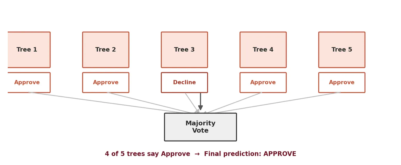
Builds many decision trees, each trained on a slightly different random sample of data and features, so the trees make different mistakes. The final prediction is made by voting (classification) or averaging (regression). This makes Random Forests much more stable than a single tree and reduces overfitting. Therefore, it is a strong default model for structured datasets, handling nonlinear patterns, interactions, and mixed feature types well. Figure 11 shows this voting process: each tree reaches its own answer independently, and the majority answer becomes the forest's final prediction. Note: more advanced tree ensembles such as gradient boosting and XGBoost (Section 4.5) exist. They still combine many trees, but the trees are built one after another, each one correcting the previous trees' errors, rather than voting independently like a Random Forest.
Real-world: fraud detection at banks, disease prediction, customer churn, manufacturing defect detection, clinical trial analysis
Use it when: you have structured, tabular data and want a strong, low-maintenance default that performs well without much tuning.
Think twice when: you need one readable rule path per prediction, very fast predictions on limited hardware, or the extra accuracy that a carefully tuned boosting model can provide.
4.5 Gradient Boosting & XGBoost: Learning from Mistakes, One Tree at a Time
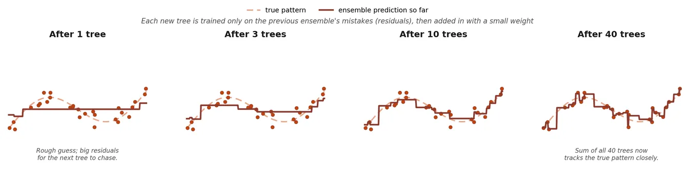
Builds many decision trees too, but unlike Random Forest, the trees are not independent: they are grown one after another, and each new tree is trained specifically on the mistakes (technically, the residuals, or more precisely the gradient of the loss function) that the trees before it made. Each tree's prediction is then added into a running total with a small weight (the learning rate), so the ensemble corrects itself gradually, round by round, instead of voting all at once like a Random Forest. Gradient boosting is the general algorithm; XGBoost is one particular implementation of it, and the best known. It adds L1/L2 regularization to the training objective, uses second-order gradient information, grows and prunes its trees efficiently, and has a built-in rule for handling missing values, which is a large part of why it became one of the most widely used models for structured-data competitions and production systems. Those specifics belong to XGBoost rather than to boosting in general: LightGBM and CatBoost are two other widely used implementations of the same underlying idea with different trade-offs, LightGBM usually being fastest on large datasets and CatBoost handling categorical features with the least preparation, so in practice "gradient boosting" almost always means one of these three. Because each tree is chasing the previous trees' errors, boosted models can reach very high accuracy on structured data, but they are also more prone to overfitting than Random Forest if the learning rate, tree depth, and number of trees are not controlled carefully. Figure 12 shows this residual-correction process across several rounds of boosting.
Real-world: credit risk scoring, click-through-rate prediction for ads and search ranking, insurance claim prediction, demand forecasting, structured-data competitions (Kaggle-style)
Use it when: you want the strongest typical accuracy on structured, tabular data and you have the time to tune the learning rate, tree depth, and number of trees.
Think twice when: tuning time is not available, the data is very noisy, since boosting chases noise harder than a Random Forest does, or simple interpretability is a requirement.
4.6 SVM (Support Vector Machine): Find the Widest Gap
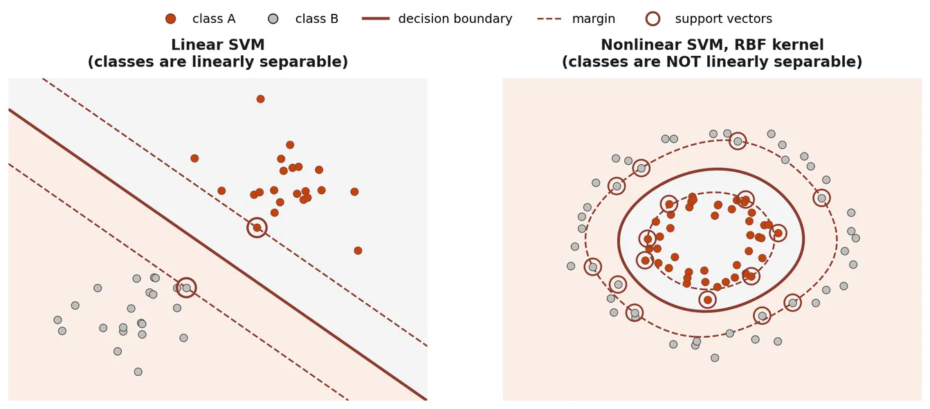
This model finds a decision boundary that separates classes with the widest possible margin. The training points closest to that boundary are called support vectors, because they are the only points that fix where the boundary sits: every other training point could move slightly without changing it at all. SVMs are useful when the dataset is not huge but the number of features is high, such as text classification or gene-expression data. The basic version is a linear SVM, where the boundary is a straight line (or, with more than two features, a flat hyperplane), and it works well whenever the classes are roughly separable by a straight cut. When they are not, a nonlinear SVM uses the kernel trick (a mathematical shortcut that lets the SVM measure similarity as if the data had extra, curved dimensions, without ever actually computing them) to bend that boundary into a curve, at the cost of more hyperparameters to tune (which kernel, and how curved) and slower training. SVMs can be powerful, but may become slow on very large datasets and usually need scaled features. Figure 13 shows both cases side by side, with the support vectors circled in each.
Real-world: genomics (gene expression classification), text classification, medical image classification when data is limited, handwriting recognition
Use it when: the dataset is small or medium but has many features, such as text or gene expression data, and a reasonably clear margin between the classes is plausible.
Think twice when: the dataset is large, since training scales poorly with the number of examples, you need well-calibrated probabilities directly, or you cannot scale the features first.
4.7 KNN (K-Nearest Neighbors): You Are Your Neighborhood
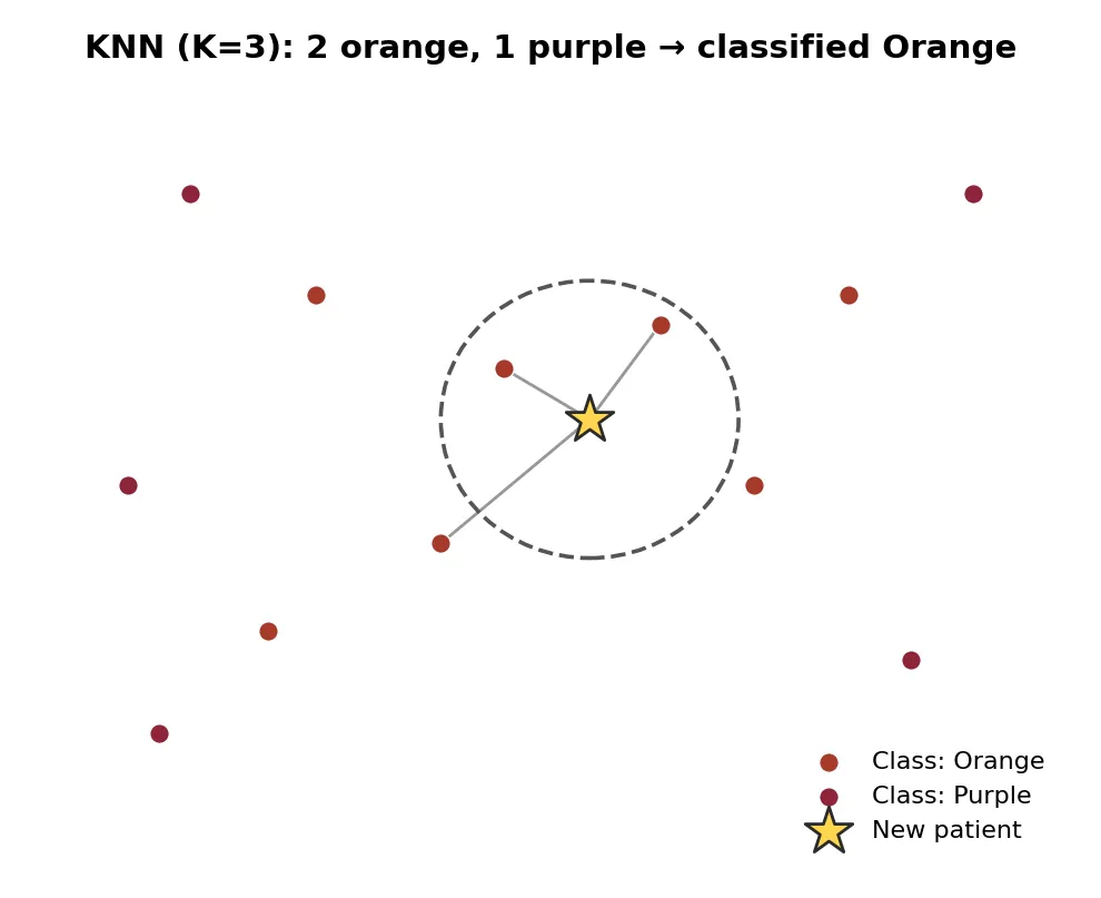
One of the simplest ML ideas, and it does not really train a model in the usual sense: it stores the training examples and compares each new example to them. For classification, it looks at the K most similar neighbors and takes a vote; for regression, it averages their numeric values. KNN is intuitive and useful for small datasets, but it becomes slow with many examples and depends heavily on good distance measures and normalized features. Figure 14 shows a new example being classified by a simple majority vote among its K=3 nearest neighbors.
Real-world: recommendation systems (users similar to you liked X), anomaly detection, medical case-based reasoning, image retrieval
Use it when: the dataset is small, "similar examples" is a meaningful idea for your problem, and you want a baseline with essentially no training step at all.
Think twice when: the dataset is large, since every single prediction searches the whole training set, the feature count is high, since distances lose meaning in many dimensions, or the features are unscaled.
4.8 K-Means Clustering: Find Natural Groups Without Labels
While others are supervised models, this one is an unsupervised model: it works without labels. It tries to find K natural groups by placing cluster centers in the data and assigning each point to the nearest one; the centers move repeatedly until the groups become stable. Useful for exploration, segmentation, and discovering structure before you know the exact labels. The user must choose K, and results can change if features are not scaled or if the clusters are not roughly compact and separated. Figure 15 shows the result on a dataset with no labels at all: the algorithm still recovers three sensible customer groups purely from how the points cluster in space.
Real-world: customer segmentation (budget vs premium buyers), patient subgroup discovery, market research, anomaly detection, gene expression analysis
Use it when: you have no labels and want a fast first look at whether the data falls into a few compact, roughly round groups.
Think twice when: the groups are elongated, nested, or very different in size and density, or when you have no principled way to choose K.
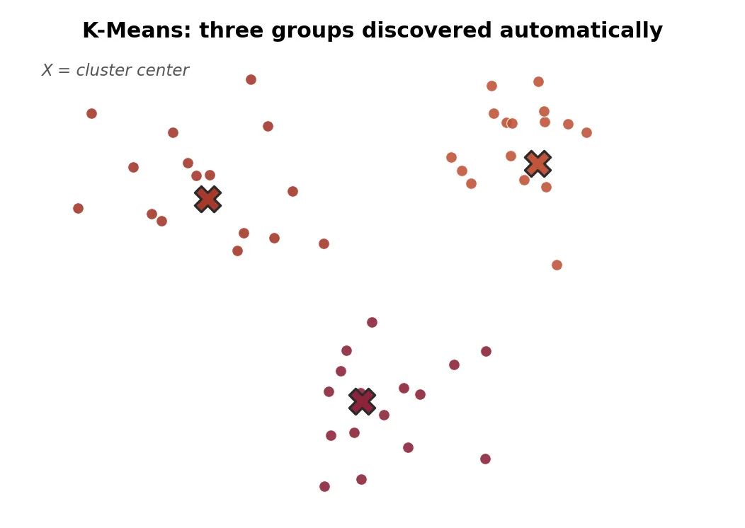
Table 1 pulls the seven non-neural models from this section into one place, together with XGBoost (Section 4.5), so they are easy to compare on a few practical properties before moving to neural networks in Section 5: whether the model can select useful features by itself while training, whether it needs normalized or scaled input to work well, whether it produces a score suitable for a ROC curve, and how it compares on interpretability, nonlinearity, and training speed.
Model | Inherent feature selection | Needs normalized / scaled input | ROC-curve-ready output | Interpretability | Handles nonlinear patterns | Training speed |
|---|---|---|---|---|---|---|
Linear Regression | No (add L1/Lasso for this) | Helps, not required for the closed-form fit | N/A (regression, not classification) | High | No (linear only) | Very fast |
Logistic Regression | No (add L1/Lasso for this) | Yes, especially with regularization | Yes, outputs a probability directly | High | No (linear boundary) | Very fast |
Decision Tree | Yes (splits reveal important features) | No (splits on thresholds, not distance) | Yes, via leaf class proportions | High | Yes | Fast |
Random Forest | Yes (feature-importance scores) | No | Yes, via vote proportions | Medium | Yes | Medium |
XGBoost | Yes (gain-based importance scores) | No | Yes, via predicted probability | Medium | Yes | Fast (optimized gradient boosting) |
SVM | No | Yes, strongly (margin-based) | Yes, via the decision function (calibrate for true probabilities); though not generally used though | Low to medium (kernel-dependent) | Yes (with kernels) | Slow on large data |
KNN | No | Yes, strongly (distance-based) | Yes, via neighbor vote share | Medium | Yes | Slow at prediction time |
K-Means | N/A (unsupervised, uses all given features) | Yes, strongly (distance-based) | N/A (unsupervised, no labels/threshold) | Medium | Only with kernel variants | Fast |
5. The Neural Network Core
Neural networks sound intimidating, but their core idea is very simple. A neural network is built from connected neurons that learn weights, biases, and activation functions. These let the model transform input numbers step by step until it can make a prediction. Architectures such as CNNs, RNNs, LSTMs, and Transformers (Section 6) all use this same foundation; what changes is how the neurons are connected and what kind of data the architecture is designed to handle.
5.1 One Neuron: The Simplest Possible Unit
A single neuron receives input numbers, multiplies each by a learned weight, adds a learned bias, then passes the result through an activation function. The weight controls how strongly an input matters; the bias shifts the decision point; the activation function lets the neuron create nonlinear patterns instead of only straight-line relationships. One neuron is simple, but many neurons combined can represent very complex functions.
The single-neuron formula (that is literally all it is)
z = w1*x1 + w2*x2 + w3*x3 + bias → output = activation(z)
Weighs decide how strongly each input affects the neuron. The bias shifts the result up or down. The activation function adds nonlinearity, which is what allows the network to learn curved and complex patterns: without it, even many stacked layers would behave like one large linear equation.
Figure 16 compares the three activation functions you will see most often. ReLU keeps positive values unchanged and zeroes out negative ones, which trains quickly and is the default choice for hidden layers. Sigmoid squashes any input into a 0-1 range, which is why it appears at the output of binary classifiers. Tanh behaves similarly to sigmoid but is centered at 0, which some older sequence models rely on.
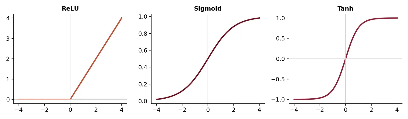
Activation | What It Does | Common Use |
|---|---|---|
ReLU | Keeps positive values and turns negative values into zero. | Most hidden layers, because it is simple and trains well. |
Sigmoid | Squashes any value into a number between 0 and 1. | Binary classification output, when the model predicts a probability. |
Tanh | Squashes values between −1 and +1. | Older sequence models, and cases where centered outputs help. |
5.2 Stack Neurons into Layers: Now It Gets Powerful
A layer is a group of neurons working at the same stage of the network. When neurons are stacked into layers, each layer transforms the input into a more useful representation: early layers often learn simple patterns, later layers combine them into more abstract ones. In a basic Multilayer Perceptron (MLP), each neuron in one layer connects to every neuron in the next layer. Training adjusts all those weights, so the final output moves closer to the correct answer. Figure 17 shows this layout: data enters on the left, flows through one or more hidden layers, and produces a prediction on the right, with every connection carrying its own learned weight.
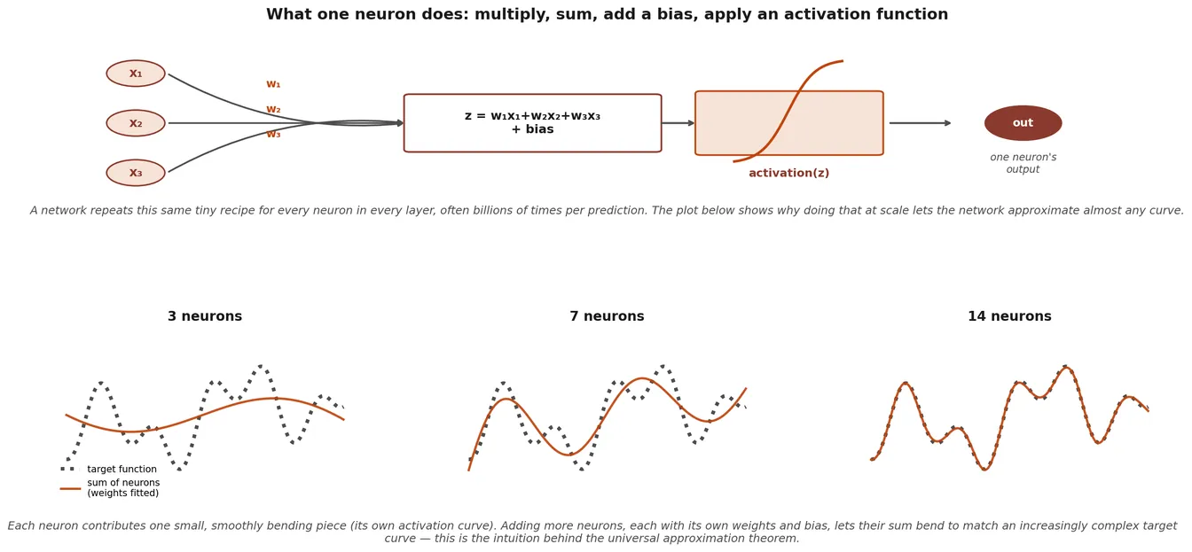
So basically, in my view, what neural-network-based models do under the hood is multiply and sum thousands, millions, or even billions of numbers (and pass the results through activation functions to add nonlinearity). When you do this much computation at such a super large scale, it can approximate almost any function (my own take on it). Different architectures and training approaches exist to make this process dramatically more efficient, which is how we end up with systems like ChatGPT and Claude, but underneath the code, this same simple math is what powers the neural networks.
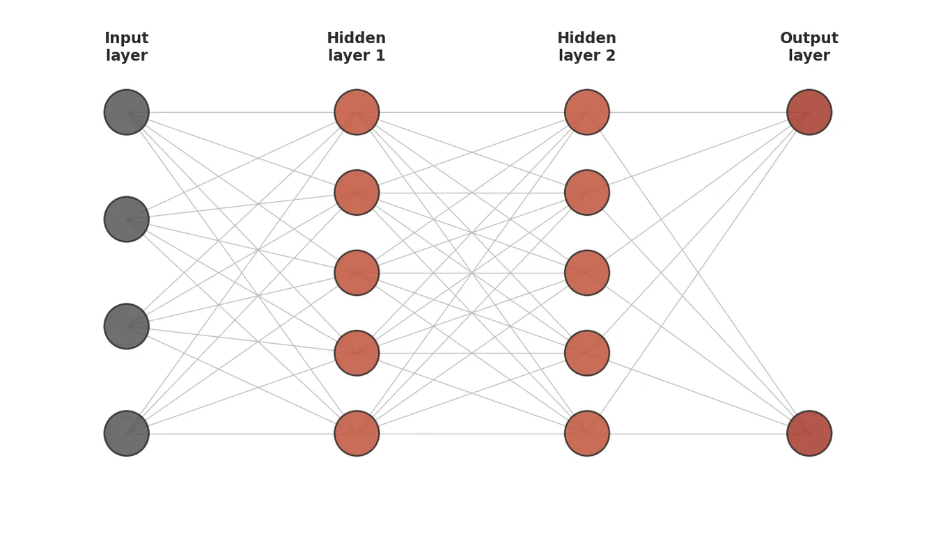
Figure 18 below zooms into a single neuron's math and shows why repeating it at scale lets a network approximate almost any function.
5.3 How Training Works: The Three-Step Loop
So here, basically we need to find all the right numbers in those multiplications and summations that connect each neuron with other neurons. This is done as follows:
Step 1: Forward pass: Feed an example through the network and produce a prediction; no weights change yet.
Step 2: Calculate loss: Compare the prediction with the correct answer and measure the error. Mean Squared Error is common for regression; Cross-Entropy is common for classification (it penalizes a confident wrong answer more heavily than an uncertain one).
Step 3: Backpropagation and gradient descent: Work backward through the network, estimate how much each weight contributed to the error, and nudge every weight slightly in the direction that reduces future error. Repeating this loop many times, over many examples, is how the network learns.
Training Step | Simple Meaning | What Changes |
|---|---|---|
Forward pass | The network uses the current weights to make a prediction. | No weights change yet. |
Loss calculation | The prediction is compared with the correct answer. | The model measures how wrong it is. |
Backpropagation | The error is traced backward through the network. | Each weight receives a correction signal. |
Gradient descent | Weights are nudged in the direction that lowers loss. | The network becomes slightly better for the next example. |
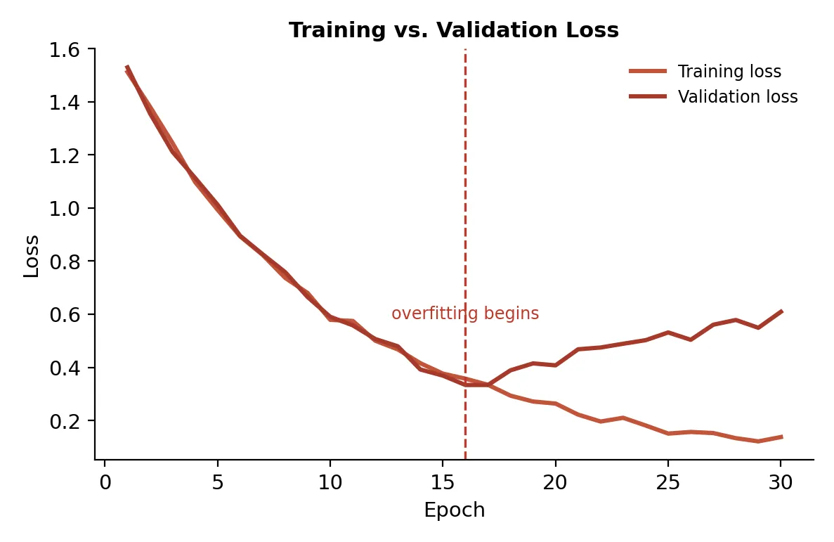
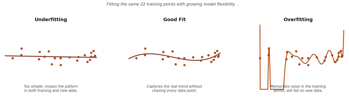
Figure 19 shows what this loop produces over many epochs: a training loss curve, where one epoch is one complete pass through the entire training dataset (Section 5.3 repeats this pass many times, adjusting the weights a little after each one). The training set is the data the model directly learns its weights from, and the validation set is a separate slice the model never learns from directly, used only to check how the model is doing on examples it has not memorized (Section 9.2 covers this split in full). Training loss should fall steadily, and validation loss should fall with it. When validation loss starts rising while training loss keeps falling, that growing gap is the signature of overfitting: the model is beginning to memorize the specific training examples, noise included, rather than learning the underlying pattern that would carry over to new data. Figure 20 shows the same idea a different way: as a model is given more flexibility to bend around the training points, it moves from underfitting, too simple to capture the real pattern, through a good fit, to overfitting, so flexible that it chases every training point, noise included, and fails on new data. This is exactly why avoiding overfitting matters: a model that overfits can look excellent during development and still perform poorly the moment it sees real, new examples. Section 9 covers the full discipline for catching this reliably, including how the training, validation, and test sets it relies on are meant to be used.
6. Neural Networks for Specific Tasks
Section 5 explained the core building blocks of neural networks: neurons, weights, biases, activation functions, layers, loss, and backpropagation. Section 6 shows how those same building blocks are arranged differently for different kinds of data. An MLP works well when the input is already a feature vector. A CNN is arranged for pixels and image-like grids. RNNs and LSTMs are arranged for ordered sequences. Transformers are arranged around attention, which helps the model relate one part of the input to other parts. The neuron is always the basic unit but the architecture just decides what kind of pattern the network can see easily.
Architecture | Best Input Shape | Main Idea | Typical Uses |
|---|---|---|---|
MLP | Feature vectors, tables | Every neuron connects to the next layer; learns patterns from prepared numeric inputs. | Tabular classification, regression, simple prediction |
CNN | Images, spectrograms | Small filters scan local regions and learn visual or frequency patterns. | Image diagnosis, defect detection, face recognition, audio spectrograms |
RNN | Sequences | Information passes from one time step to the next, so order matters. | Time series, sensor streams, simple text and audio sequences |
LSTM | Longer sequences | Memory gates help the network keep or forget information over time. | Forecasting, audio, speech, health signals, longer sensor patterns |
Transformer | Text, sequences, multimodal | Attention lets each part of the input decide which other parts are relevant. | Language models, translation, summarization, search |
6.1 CNN (Convolutional Neural Network): Made for Images
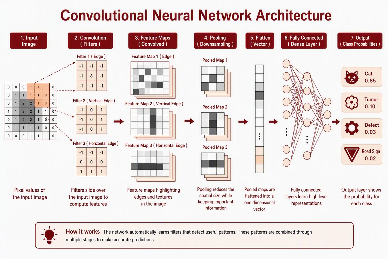
A Convolutional Neural Network, or CNN, is designed for image-like data. The input begins as a grid of pixel values. Small filters slide across nearby pixels and detect local patterns such as edges, corners, textures, and color changes. Then, these detected patterns become feature maps, which show where a pattern appears in the image. Pooling reduces the size of the feature maps while keeping the strongest signals. Finally, dense neuron layers combine those learned visual features and produce output probabilities such as cat, tumor, defect, or road sign. This is why CNNs are useful for images: they learn from local pixel neighborhoods instead of treating every pixel as unrelated. Figure 21 walks through the full pipeline.
Real-world: medical imaging (reading X-rays, detecting tumors), facial recognition, self-driving cars, quality control in manufacturing, satellite imagery analysis
Use it when: the input is an image or any grid where nearby values are related, such as pixels or spectrograms, and you have either enough labeled data or a pretrained model to fine-tune.
Think twice when: the data is a table of unrelated columns, since there is no local structure for filters to exploit, or you have only a few hundred labeled examples and no suitable pretrained model.
6.2 Audio Processing: Sound as a Spectrogram Image
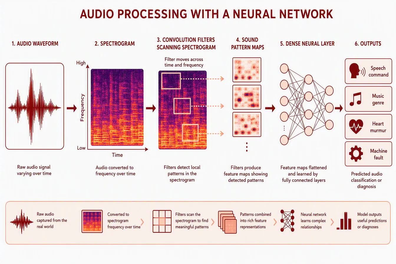
Audio is a signal that changes over time. The waveform shows sound pressure moving up and down, but this raw shape is hard to interpret directly. A spectrogram turns the same sound into an image-like grid where the horizontal direction is time and the vertical direction is frequency where bright or dark regions show which frequencies are active at each moment. Once audio is represented as a spectrogram, a CNN can scan it just like an image, and its filters can learn patterns such as rhythm, pitch changes, repeated sounds, machine noise, speech sounds, or heart murmurs. The spectrogram is not the final answer of the question of what input to use, but it is a useful view of the audio that helps the neural network learn sound patterns more efficiently. Figure 22 shows the full pipeline.
Real-world: speech recognition (Siri, Alexa), music genre classification, heart murmur detection, noise cancellation, Shazam-style music identification
Beginner note: is a spectrogram raw data or a hand-made feature?
A spectrogram is not a small, hand-made feature like "average pitch" or "loudness." It is a general-purpose mathematical view of the same audio signal, though not a choice-free one: the window length and frequency resolution are set by a human and trade detail in time against detail in frequency. The human chooses this view, but the model still has to learn which shapes, frequency changes, and repeated patterns actually matter. This is why spectrograms sit between raw audio and learned features: they organize the sound, but they do not decide the answer for the model.
6.3 Recurrent Neural Networks and Long Short-Term Memory Networks
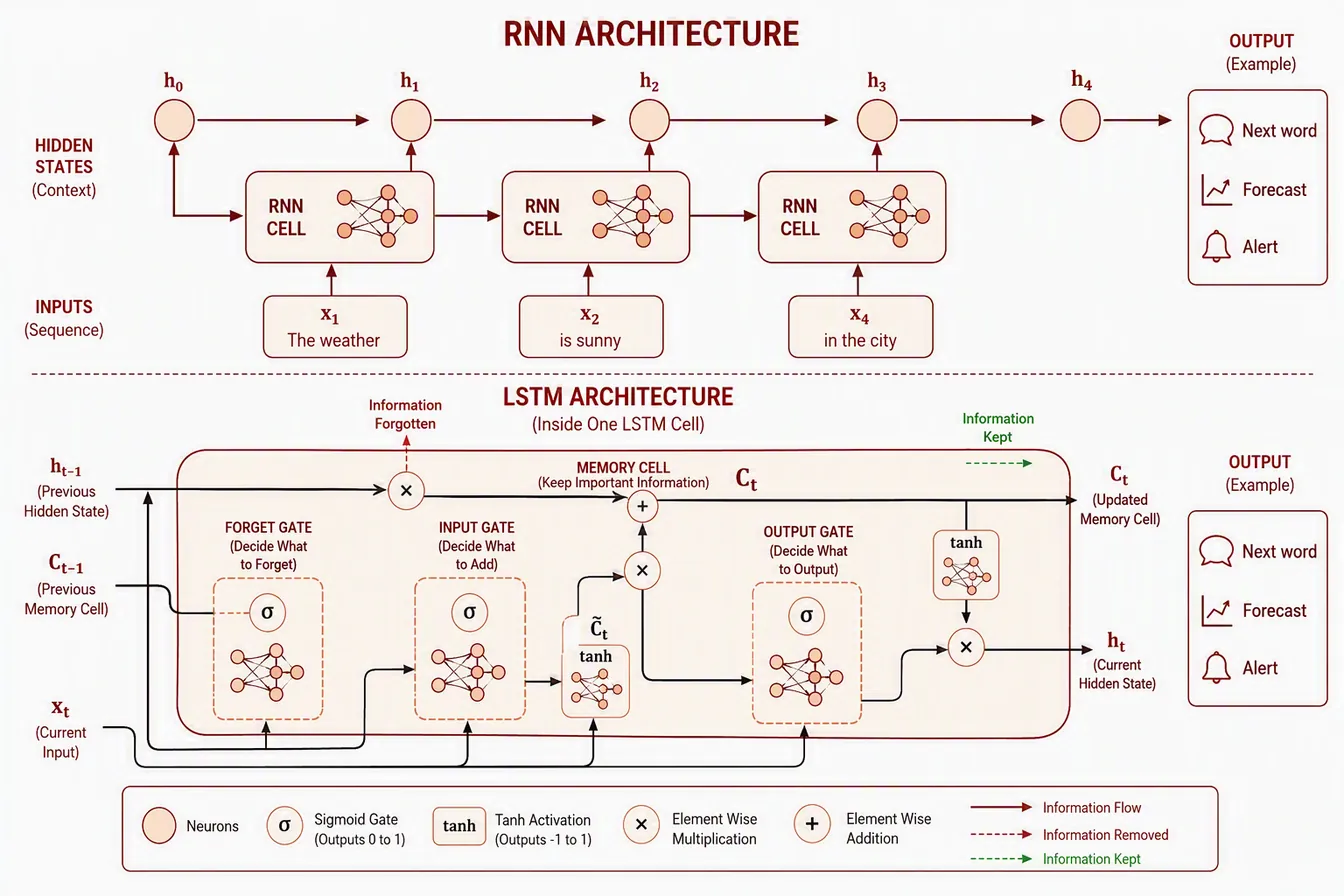
A Recurrent Neural Network, or RNN, is designed for ordered data. It reads one step at a time: the first word, then the second word, then the third; or one sensor reading, then the next. After each step it carries a hidden state forward, a small memory of what has happened so far. The weakness of a simple RNN is that it can forget information from many steps earlier. A Long Short-Term Memory network, or LSTM, fixes this with gates: a forget gate decides what old information to drop, an input gate decides what new information to add, and an output gate decides what to pass forward. This makes LSTMs useful for longer sequences such as forecasting, speech, medical signals, and robot sensor streams. Figure 23 shows both architectures side by side.
Use it when: order matters, the sequences are short to moderate in length, or you need a small model that processes a stream one step at a time as it arrives.
Think twice when: the sequences are long and the important relationships span large distances, which attention handles better, or when training speed matters, since recurrence is sequential and hard to parallelize.
6.4 Transformers and Attention
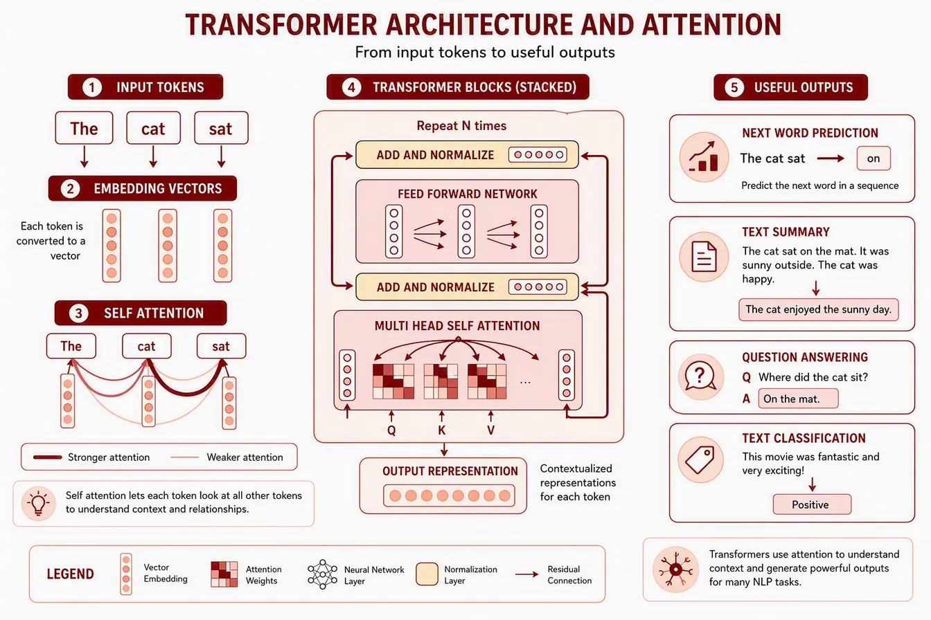
A Transformer is designed to compare many parts of an input at the same time, rather than walking through them in order. The input is first cut into tokens: words or word pieces for text, patches for an image, short frames for audio. Each token becomes an embedding vector, which is a list of numbers standing for its meaning (Section 6.5). Because nothing in this setup inherently knows what order the tokens arrived in, a positional encoding is added to each embedding so the model can still tell the first word from the fifth.
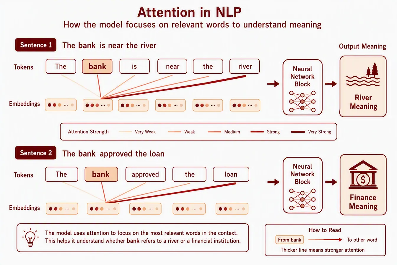
Self-attention is the core operation. For every token, the model compares that token against all the others and produces a set of relevance weights, then rebuilds that token's representation as a weighted blend of the tokens it found relevant. This is exactly why context can change meaning: the word "bank" ends up blended with "river" in one sentence and with "loan" in another, so its vector after attention is not the same vector in the two cases. Real transformers run several of these comparisons side by side, which is called multi-head attention, letting different heads track different kinds of relationships, such as grammatical role in one and topic in another. A transformer block then follows attention with a small feed-forward network, and these blocks are stacked many times, so each layer builds context on top of the previous one.
Two practical consequences follow from this design. First, because all tokens are compared at once instead of one step at a time, a Transformer parallelizes far better during training than an RNN does, which is a large part of why this architecture, and not recurrence, scaled to today's model sizes. Second, that same all-pairs comparison means the computation grows roughly with the square of the sequence length, which is why very long inputs get expensive and why a great deal of research goes into making attention cheaper. This architecture is the foundation of modern large language models, translation systems, summarizers, search systems, and multimodal models that combine text with images, audio, or video. Figure 24 walks through the pipeline from tokens to outputs.
Use it when: relationships between distant parts of the input matter, and you have either a large dataset or a suitable pretrained model to build on.
Think twice when: the dataset is small and no pretrained model fits your domain, since transformers are data hungry, or when compute and latency budgets are tight, since attention cost grows quickly with sequence length.
6.5 NLP: Text as Numbers, Context as Attention
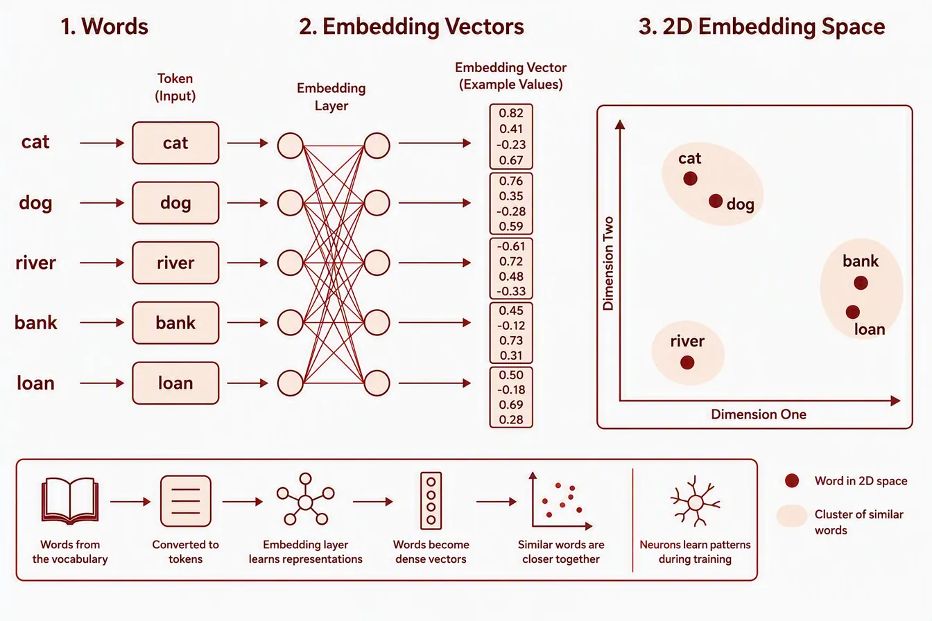
Natural language processing, or NLP, is the part of machine learning that works with text. Text cannot enter a neural network as ordinary words, so it first becomes numbers. Each word or token becomes an embedding vector which is a list of numbers that represents meaning. Similar words tend to have similar vectors, which is why "cat" appears near "dog", and "bank" appears near "loan" when used in a finance context (Figure 25). As mentioned before, attention then lets the model use surrounding words to decide which meaning is intended: in one sentence "bank" connects strongly to "river"; in another, it connects strongly to "loan" (Figure 26). This is the key beginner idea behind modern NLP: embeddings turn words into numbers, and attention uses context to decide what those numbers mean in a given sentence. I could explain this section right before transformers, but since transformers used in other tasks as well, I explained transformers before this one.
Real-world: ChatGPT and other language models, Google Search, GitHub Copilot, medical record summarization, machine translation, sentiment analysis, document classification
Why the architectures differ
In a basic MLP, every neuron connects to every neuron in the next layer: this works well for feature vectors, but does not directly respect the structure of images, sound, or language. A CNN connects neurons to small local regions, which makes it strong for images and spectrograms. An RNN processes a sequence step by step, which helps when order matters, and an LSTM improves on this by keeping useful information for longer. A Transformer uses attention, so each word, image patch, or time step can decide which other parts are most relevant. The core operation is always the same, which is the learned weights and transformations, but the connection pattern changes for each data type. When you go deeper into ML, you will see many different kind of architecture and models, but they will work similarly under the hood through neurons. And it is very fun to discover different architectures. You can even come up with your own! One thing that I did not mention, there are also regularization methods for neural-networks as well, along with some approaches to improve convergence of training. But, you will learn them when you start to learn these topics.
7. Reinforcement Learning: Learning by Trial and Error
Reinforcement learning is another major area of machine learning, but it works differently from the supervised and unsupervised ideas explained in Section 1.1. In supervised learning, the model learns from examples with correct answers. In unsupervised learning, the model looks for structure without labels. In reinforcement learning, an agent learns by taking actions in an environment and receiving rewards or penalties over time. The goal is not just to predict correctly, but to learn a good strategy for making decisions.
The core idea
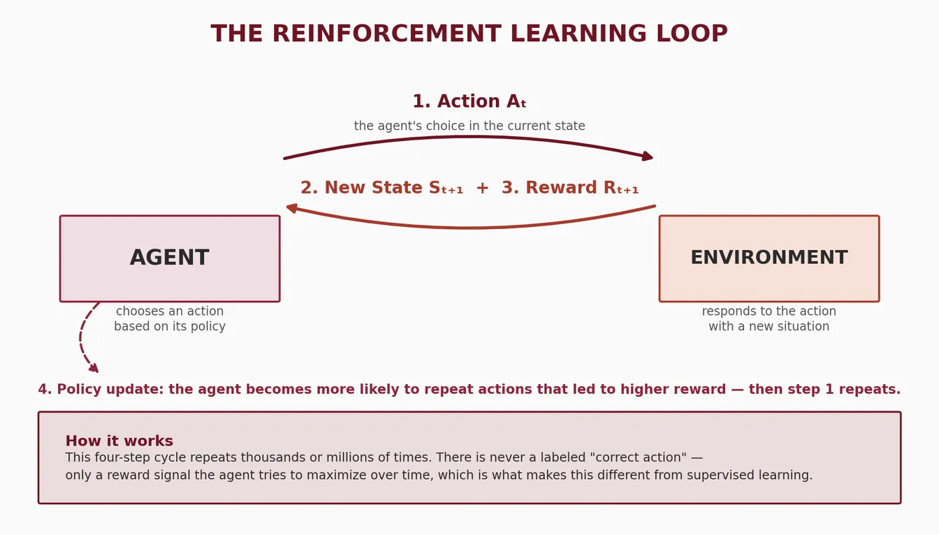
A reinforcement learning system has four basic parts: an agent, an environment, actions, and rewards. The agent chooses an action; the environment responds with a new state and a reward. Over many trials, the agent learns which actions lead to better long-term outcomes. This is why reinforcement learning is especially useful for control, planning, games, robotics, and any system where one decision changes what happens next.
7.1 How Reinforcement Learning Differs from Other ML Tasks
Learning Type | What the Model Learns From | Main Goal |
|---|---|---|
Supervised learning | Labeled examples with known answers | Predict the correct label or number |
Unsupervised learning | Unlabeled data | Find structure, groups, or unusual cases |
Reinforcement learning | Rewards and penalties from actions | Learn a strategy that gives high long-term reward |
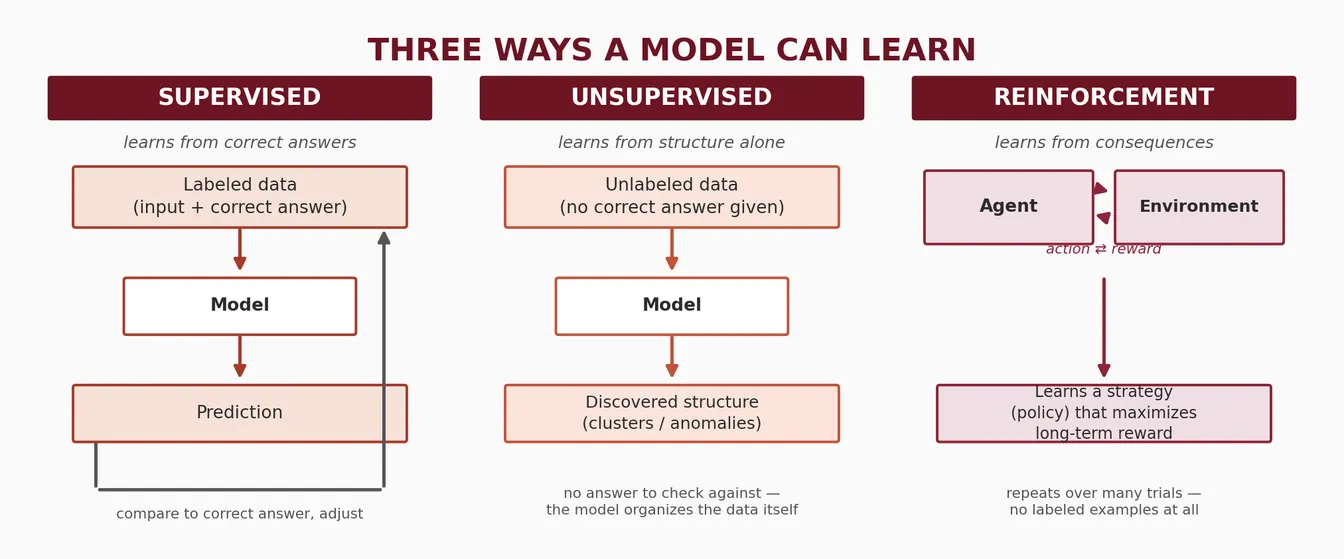
Figure 27 places the three learning types side by side. Supervised learning consumes labeled examples and outputs a predicted label or number. Unsupervised learning consumes unlabeled data and outputs discovered structure. Reinforcement learning consumes rewards generated by its own actions and outputs a strategy: the loop closes back on itself in a way the other two do not.
7.2 The Reinforcement Learning Loop
Step | What Happens | Example |
|---|---|---|
State | The agent observes the current situation. | A robot sees its position, nearby objects, and battery level. |
Action | The agent chooses what to do next. | The robot moves forward, turns, stops, or picks up an object. |
Reward | The environment gives feedback. | The robot gets a positive reward for reaching the goal and a penalty for hitting an obstacle. |
Policy update | The agent adjusts its strategy based on what happened. | The robot becomes more likely to choose actions that helped it reach the goal. |
Figure 28 draws this table as a loop, which is the more natural way to think about it: the agent observes a state, takes an action, the environment returns a reward and a new state, the agent updates its policy, and the cycle repeats, often thousands or millions of times before the policy becomes good.
7.3 What Is Actually Inside the Agent: A Table or a Neural Network
One thing this loop leaves open is what the agent actually is. Reinforcement learning describes how a model is trained, by acting, observing the reward, and adjusting, not what kind of model is doing the acting. The agent's policy, meaning its rule for choosing an action in a given state, can be stored in two very different ways, and Figure 29 shows both.
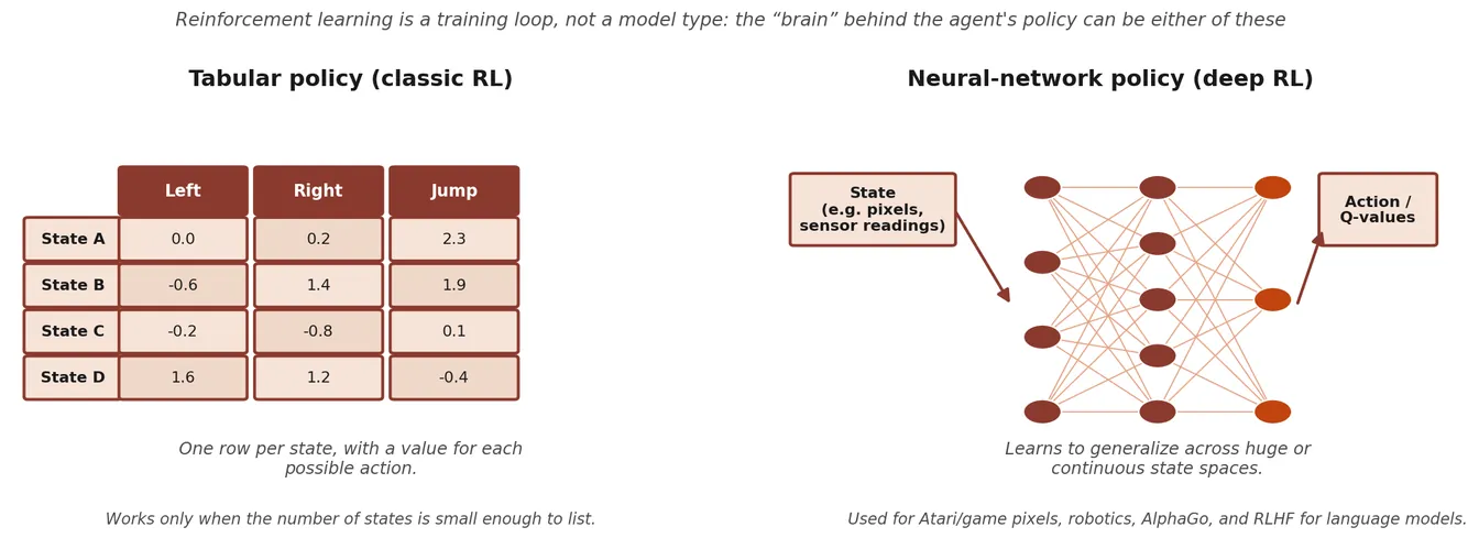
The simplest version is a lookup table, and it contains no neurons at all. Classic methods such as Q-learning keep one row per state and one column per action, holding an estimated value for each combination. The agent picks the highest-value action available in its current state, and every reward nudges the matching number up or down. This works well when the number of distinct states is small enough to list, such as a grid world, a simple board game, or a small set of machine operating modes, and it is how reinforcement learning was mostly done for decades.
The table stops working the moment the state becomes something like a camera frame, a continuous joint angle, or a full page of text, because there is no row for "this exact image" and there never will be. This is where neurons enter. A neural network replaces the table: it takes the state as input and outputs either the action to take (a policy network) or the estimated value of each action (a value network, as in a Deep Q-Network, or DQN). It is trained with the same forward pass, loss, and backpropagation loop described in Section 5.3. What changes is where the training signal comes from: rewards earned through interaction, rather than a fixed set of labeled examples. This combination is called deep reinforcement learning, and it is what sits behind systems that learn to play games from raw pixels, robot control policies, AlphaGo, and the reinforcement learning stage used to align large language models (Section 7.4).
So neurons are not a required ingredient of reinforcement learning. They are one option for the agent's policy, and the option you reach for once the state space is too large or too continuous for a table to cover. Everything else in the loop, the states, actions, rewards, and policy updates, works the same way either way.
7.4 How the Agent Actually Learns: Q-Learning and Its Relatives
Section 7.3 said the agent stores a policy, but not how the numbers in that policy become good. The usual starting point is a value, almost always written Q, attached to every pair of a state and an action. A Q-value answers one question: if I am in this state and take this action, how much total reward should I expect from here on, assuming I keep behaving sensibly afterwards? If those numbers are right, acting well becomes trivial. Look up the current state, and take the action with the highest Q-value.
Q-learning is the method that fills that table in, and its update is simple enough to say in one sentence. The agent takes an action, sees the reward it got and the new state it landed in, then asks what the best Q-value available from that new state is. The reward plus that best next value is a better estimate of what the original action was worth than the number currently stored, so the stored number is nudged a fraction of the way toward it. Repeat a few hundred thousand times and the estimates settle. Two knobs control the process: the learning rate decides how big each nudge is, and the discount factor decides how much a reward far in the future counts compared with one right now, so a discount near 1 makes the agent patient and a low one makes it greedy for immediate reward.
The interesting part is that nobody ever tells the agent which early moves were good. At first only the square next to the goal earns a real reward, so only its value rises. The next time the agent passes through the square before that one, it gets updated toward its now-valuable neighbour, and so the value seeps backward, one step per visit, until even the starting square knows which direction leads to the reward. Figure 30 shows exactly this happening on a small grid.
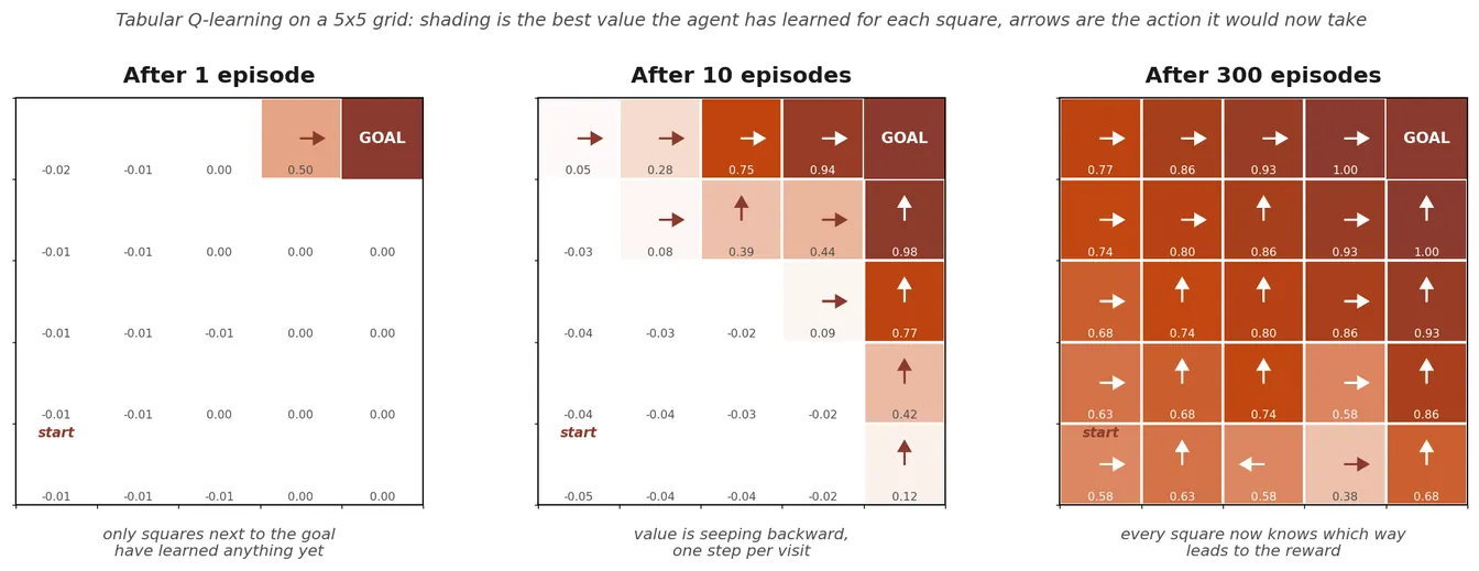
One problem hides inside "take the action with the highest value." At the start every value is wrong, so an agent that always takes its current best guess will keep repeating the first mediocre path it stumbled into and never discover the better one. This is the exploration versus exploitation trade-off, and the standard fix is deliberately crude: epsilon-greedy. Most of the time take the best known action, and with a small probability, epsilon, take a random one instead. Epsilon usually starts high and decays as learning progresses. Exploring costs reward in the short run, and it is the only way to find out what you do not already know.
Q-learning is described as off-policy, because it updates toward the best action available in the next state even when the exploring agent actually took a different one. Its on-policy sibling, SARSA, updates toward the action the agent genuinely took next instead. The practical difference is temperament. SARSA learns a route that accounts for its own occasional random moves, while Q-learning learns the optimal route and assumes the exploring will stop eventually. It is the classic reason THAT a SARSA agent walks a little further from the cliff edge.
When the table is replaced by a neural network (Section 7.3), this same idea carries over as a Deep Q-Network, with two additions that keep training stable. “Experience replay” stores past transitions in a buffer and trains on random samples drawn from it, so the network is not fed a stream of nearly identical consecutive frames. “A target network” keeps a slightly out-of-date copy of the weights for computing the "best next value" part of the update, so the target the network is chasing does not move every single step.
Value-based methods have one real weakness: picking the highest-valued action means comparing every action, which is awkward when actions are continuous, such as a steering angle or a joint torque. Policy-gradient methods skip the value table and adjust the policy directly, raising the probability of action sequences that turned out well and lowering it for the ones that did not. Actor-critic methods run both ideas at once: an actor that chooses actions, and a critic that estimates how good the current situation is, with the critic's judgment used to train the actor. PPO, short for Proximal Policy Optimization, is the actor-critic variant you will meet most often in practice, and it is the algorithm behind the reinforcement learning stage used to fine-tune large language models from human feedback.
One last distinction is worth knowing. Everything above is model-free: the agent learns purely from what happened, with no idea how the environment works internally. A model-based agent also learns, or is given, a model of the environment, and can then plan by simulating moves before committing to one. That usually needs far less real experience, which matters when experience is slow or expensive to collect, such as on a physical robot. AlphaGo is the famous hybrid, combining learned value and policy networks with a search that plays out possible continuations before choosing a move. Table 2 summarizes the whole family.
Method | What it learns | Best suited to | Note |
|---|---|---|---|
Q-learning (tabular) | A value for every state and action pair | Small, countable state spaces | Off-policy. The classic starting point |
SARSA | The same table, updated with the action actually taken | Cases where behaviour during learning matters | On-policy. Learns a more cautious route |
DQN | A network predicting Q-values from the state | Large or raw inputs, such as pixels | Adds experience replay and a target network |
Policy gradient (REINFORCE) | The policy itself, directly | Continuous actions | Simple idea, but noisy and slow to train |
Actor-critic (PPO and others) | A policy and a value estimate together | Most modern applications, including RLHF | The practical default today |
Model-based (AlphaGo style) | A model of the environment, plus planning on top | When simulating moves is possible | Needs far less real experience |
Hey, but what about the reward? What is it and how is it decided?
The reward is just a number. After each action, the environment hands the agent a single value like +1, 0, or -0.02, and that number is the only feedback the agent ever gets. Who decides that number? A human does. The reward function is written by the person setting up the problem, before any learning happens. It is not learned, and it is not discovered in the data. It is a rule that says "when this happens in the environment, emit this number." The environment is usually a piece of code (a game engine, a physics simulator, a market simulator, or a real robot plus some sensor logic), and the designer adds the line that converts what just happened into a score.
Some real examples of what that rule looks like:
In chess or Go, +1 for winning, -1 for losing, 0 for a draw, and exactly 0 for every single move in between. In Atari games, the reward is just the change in the game's own score, which is convenient because the game already computes it. For a walking robot, something like: plus the distance moved forward this timestep, minus a small amount for the energy the motors used, minus a large amount if it falls over. In the grid world in your Figure 30, it is +1 for reaching the goal and -0.02 for every step taken, and that tiny negative is what makes the agent prefer short routes instead of wandering. For a recommender, +1 if the user actually watched the thing to the end, and nothing or negative if they bounced off immediately. For data center cooling or traffic lights, the negative of energy consumed or total waiting time.
Three things follow from this that are worth knowing.
A reward is not a label. In supervised learning the data tells the model "the correct answer here was 7". A reward never says that. It says "what you just did scored 0.3" and stays silent about what would have scored better. That single difference is why reinforcement learning needs exploration at all: the only way to find out whether another action was better is to try it.
Rewards can be sparse or dense, and sparse is brutal. A chess agent that only gets a signal on the final move has to figure out which of its forty moves deserved the credit. A dense reward, meaning a small signal at every step, learns far faster. Deliberately adding intermediate rewards to help is called reward shaping, and it is one of the most practical skills in RL.
The agent optimizes exactly what you wrote, not what you meant. This is the famous failure mode. In a boat racing game, an agent rewarded for collecting score powerups learned to drive in circles hitting the same respawning powerups forever instead of finishing the race, because that genuinely earned more points. A cleaning robot rewarded for "no mess detected" can learn to knock the bin over so it has something to clean again, or simply to stop looking. This is called reward hacking or specification gaming, and it is why writing the reward function is often the hardest part of an RL project, harder than choosing the algorithm.
7.5 Common Reinforcement Learning Uses
Robotics: learning movement, grasping, navigation, and control policies through repeated interaction with an environment.
Games: learning strategies by playing many rounds and improving from wins, losses, and rewards.
Recommendation systems: choosing which item to show next while balancing short-term clicks with long-term user satisfaction.
Operations and control: optimizing traffic lights, warehouse routing, energy systems, inventory decisions, or scheduling policies.
Large language model alignment: improving model behavior using feedback signals from humans, preference models, or reward models.
Simple way to remember it
Supervised learning learns from correct answers. Unsupervised learning finds patterns without answers. Learning reinforcement learns from consequences. It is most useful when the model must make a sequence of decisions and the value of an action depends on what happens later.
8. Wrap-Up: When to Use What
Non-Neural Model | Neural Network | |
|---|---|---|
Data type | Structured / tabular (spreadsheets, databases) | Unstructured (images, audio, raw text) |
Dataset size | Small to medium (under ~100k rows) | Large (100k+, ideally millions) |
Interpretability | Yes: explain every prediction (medical, legal) | Not always required in the application |
Training time | CPU, seconds to minutes | GPU, hours to weeks |
Feature work | You provide meaningful features | Model can learn features from raw input |
Example tasks | Patient risk, fraud, churn, price forecasting | Tumor detection, voice assistant, chatbot, translation |
Practical rule of thumb
Especially for structured data, start with a Random Forest (Section 4.4) or XGBoost. XGBoost is a gradient-boosted-tree model: like a Random Forest, it combines many decision trees, but instead of growing them independently and voting, it grows them one after another, with each new tree specifically trained to correct the mistakes the trees before it made. Both are fast, robust, and handle messy real-world data extremely well. Only switch to neural networks when: (1) your data is images, audio, or raw text; (2) you have a very large dataset and simpler models have plateaued; or (3) the task requires learning complex hierarchical representations.
Put simply: for classification and regression on structured, tabular data, start with a non-neural model. It is simpler, cheaper to train, and usually matches or beats a neural network there anyway. For harder, unstructured tasks such as images, audio, and NLP, go straight to a neural network unless you specifically want the simplicity and low computational cost of a non-neural approach and are willing to trade away some accuracy for it.
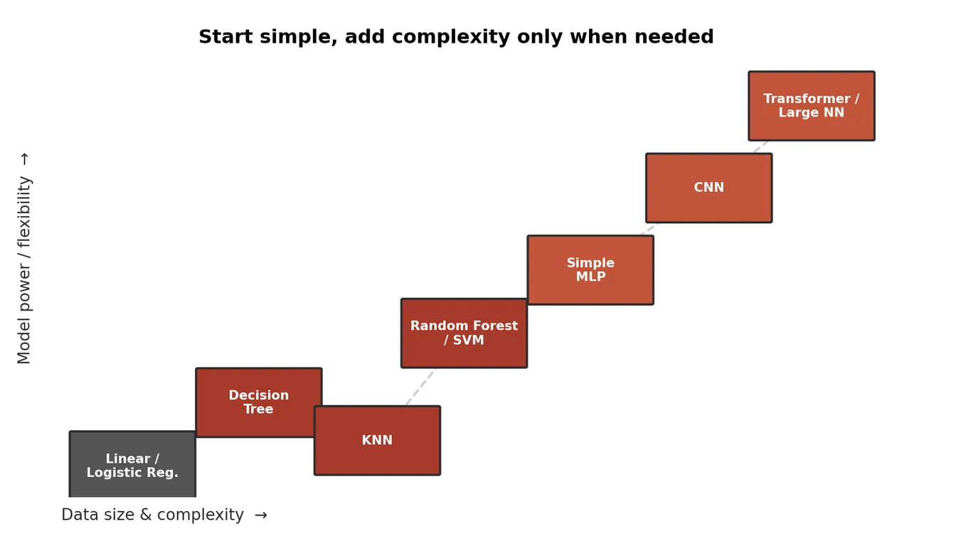
9. Evaluating Model Performance
Every model in this guide such as non-neural or neural, classification or regression eventually must answer one question: how do you actually know if it is any good? Therefore, I added this section in the end after you know the models and which model to choose for your work. This section covers the standard discipline for answering that honestly. It applies equally to every model family covered so far; only the specific metric you pick at the end differs by task.
9.1 Why Training Accuracy Can Lie to You
A model's score on the exact data that it was trained on is almost always optimistic, and sometimes wildly so. Section 5.3 introduced this problem as overfitting: given enough capacity, a model can start memorizing the specific examples it was shown including their noise and quirks, instead of learning the underlying pattern that would carry over to new cases. A fraud-detection model that scores 99.9% on the transactions it trained on might catch far fewer real fraud cases the following month, on transactions it has never seen before. The fix is not a clever trick, but it is a discipline: never judge a model using the same rows it learned from.
9.2 Splitting Your Data: Training, Validation, and Test Sets
The standard solution is to split your labeled data into three separate parts before training even begins, and to use each part for a different job only.
Set | What It's For | When You Touch It |
|---|---|---|
Training set | The model directly learns its weights, splits, or coefficients from this data. | Constantly, throughout training. |
Validation set | Used to tune hyperparameters, like tree depth or learning rate that are chosen before training rather than learned from data, and to choose between candidate models, without ever letting the model learn from it directly. | Repeatedly, during development. |
Test set | Held back completely and never looked at until the very end, then used exactly once to report an honest, final performance number. | Once, after everything else is finished. |
A useful analogy: the training set is like your homework and textbook examples, the validation set is like practice exams you use to check your understanding and adjust how you study, and the test set is like the real final exam: one you only see once, and that determines your actual, honest grade. A typical split might be roughly 60% training, 20% validation, and 20% test, though the right proportions depend on how much data you have overall.
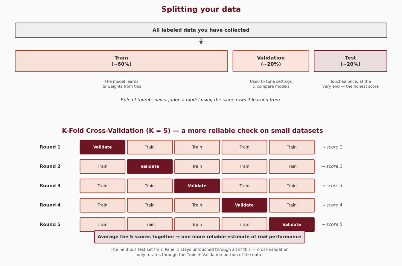
9.3 Cross-Validation: A More Reliable Read on Small Datasets
A single train/validation split has a weakness: if the dataset is small, the one validation slice you happened to carve out might be unusually easy or unusually hard by chance, giving a misleading picture of the model. K-fold cross-validation fixes this by rotating which slice of the data plays the validation role. The training-and-validation portion of the data is divided into K equal-sized folds. The model is then trained K separate times: each time, one fold is held out as validation and the rest are used for training. After K rounds, every example has been used for validation exactly once, and the K resulting scores are averaged into a single, more reliable estimate. Figure 32 shows this with K=5. The test set from Section 9.2 stays completely separate through all of this: cross-validation only rotates through the training and validation data, never the final test set.
One important nuance: a single round of K-fold cross-validation scores one fixed choice for one specific model trained with one specific set of hyperparameters. If you want to compare several candidates for different hyperparameter values, or even different model types entirely, such as a Random Forest against an SVM, you run the full K-fold cross-validation separately for each candidate, then compare their averaged scores and keep whichever one wins. Searching over many hyperparameter combinations this way is called grid search. Trying every combination in the grid works, but smarter search strategies exist that reach a good combination with far fewer training runs; they are not covered here for the sake of brevity. (Once grid search has picked a winner, it is retrained on the full training-and-validation data and evaluated once on the test set. Remember the test set itself is never used to help pick between candidates.)
Small datasets: cross-validation is especially valuable, since a single split would waste too much of the limited data on validation alone, and any one split is more likely to be unrepresentative by chance.
Large datasets: a single train/validation split is often good enough, since there is plenty of data for both parts to be representative, and cross-validation's extra training rounds cost more computing for comparatively little extra benefit.
9.4 Reading a Confusion Matrix, and Choosing the Right Metric
Section 3.3 introduced accuracy, precision, recall, F1, and ROC/PR AUC as fixes for evaluating models on imbalanced data, and they are all defined in the Glossary (Section 11). Before using them, it helps to see where they actually come from: a confusion matrix, which simply counts how a classifier's predictions land against the true answers.
Confusion Matrix
Predicted Positive | Predicted Negative | |
|---|---|---|
Actually Positive | True Positive (TP):correctly caught | False Negative (FN): missed it |
Actually Negative | False Positive (FP): a false alarm | True Negative (TN): correctly cleared |
Precision asks: of everything the model flagged positive, how much was actually positive? (TP divided by TP+FP.) Recall asks: of everything that was actually positive, how much did the model actually catch? (TP divided by TP+FN.) Accuracy simply asks what fraction of all predictions, positive and negative combined, were correct, which is exactly why it hides problems on imbalanced data, where predicting the majority class every single time can still score a high accuracy while producing zero true positives.
Task | Metric | What It Tells You |
|---|---|---|
Classification | Accuracy | Overall fraction correct. Misleading when classes are imbalanced. |
Classification | Precision | How trustworthy a positive prediction is. |
Classification | Recall | How many of the real positives the model actually caught. |
Classification | F1 Score | A single balance of precision and recall. |
Classification | ROC AUC / PR AUC | Overall separation quality across every threshold, not just one. |
Regression | MAE (Mean Absolute Error) | Average size of the error, in the target's own units. |
Regression | RMSE (Root Mean Squared Error) | Like MAE, but penalizes large errors more heavily. |
There is no single metric that is always correct: the right choice depends on the task, and especially on what a false positive costs compared to a false negative. In disease screening, missing a real case (a false negative) is usually far worse than a false alarm, so recall is prioritized. In a spam filter, wrongly blocking an important email (a false positive) may be worse than letting one spam message through, so precision is prioritized. The same logic separates the two AUC scores. ROC AUC measures how well the model ranks positives above negatives across every threshold, and it reads sensibly when the classes are reasonably balanced. PR AUC, built from precision and recall, looks only at the positive class and gives a far more honest picture when positives are rare, because ROC AUC can still look flattering when the negative class is so large that even many false alarms barely move the false positive rate. For rare-event problems such as fraud, disease screening, or failure detection, report PR AUC rather than relying on ROC AUC alone.
9.5 Data Leakage: When a Correct Split Still Lies
Even a perfectly executed split can produce a dishonest score if information about the answer leaks into the features. Leakage means the model sees something during training that it will not have at prediction time in real use. The clearest version is a column created after the fact: a discharge-reason field in a hospital dataset, or an investigation-opened flag in a transactions table. Both are wonderfully predictive and both are useless in production, because they only exist once the answer is already known.
Leakage also enters much more quietly, through preprocessing. If you compute the mean used for imputation, or the minimum and maximum used for normalization, across the whole dataset and only then split it, every training row has already absorbed a little information from the test rows, and the test score is no longer clean. The fix is an ordering rule: split first, then fit every preprocessing step on the training portion only, and apply that fitted transformation to the validation and test portions. The warning sign is an evaluation score that looks too good to be true. It usually is, and leakage is the first thing to check, which is why Section 3.2 already lists it as a question to ask during exploration.
9.6 When a Random Split Is the Wrong Split
Shuffling rows at random assumes that the rows are independent of each other and that training and test data come from the same situation. That assumption fails in three common cases, and each one needs a different kind of split.
Time series: if the task is to predict the future, a random split lets the model train on next month while being tested on last month, which is information it will never have in real use. Split by time instead, training on the earlier period and testing on the later one. Because this case is so common, Section 9.7 works through it properly.
Grouped data: when many rows come from the same source, such as the same patient, the same machine, the same customer, or the same document, a random split can put some of that source's rows in training and the rest in test. The model can then score well by recognizing the source rather than by learning the pattern you care about. Keep every row from a given source entirely on one side of the split, which is usually called a grouped split.
Genuinely new conditions: the hardest and most honest test is whether the model still works on a subject it has never seen at all, such as a new site, a new machine, a new hospital, a new season, or a new population. A model can look strong on held-out data drawn from the same sources it trained on and still fail on the next one, because it learned the quirks of the setups it saw rather than the underlying relationship. If the model is meant to be deployed somewhere new, hold out an entire source and test on that. The number it produces is usually lower than the random-split number, and it is much closer to what deployment will actually feel like.
9.7 Splitting Time Series Data in Practice
Because time-ordered data is so common, it is worth spelling out how its split actually works. The rule is that every row used for training must come from before every row used for validation or testing. You pick one or more cut-off dates and slice the timeline there, rather than sampling rows, and nothing is shuffled at any point. Figure 33 shows the shapes described below.
The simplest version is a single chronological holdout: train on the oldest stretch, validate on the middle stretch, and keep the most recent stretch as the test set. This mirrors the real situation, where you fit on everything available so far and predict what has not happened yet. It is usually the right default when the series is long enough that the final slice still holds enough examples to mean something.
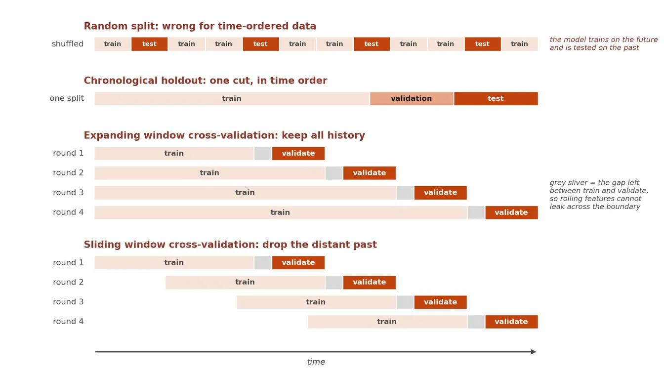
For a more reliable estimate, the cross-validation idea from Section 9.3 can be adapted, as long as the folds move forward in time instead of being drawn at random. There are two common shapes. An expanding window keeps all history and grows the training set each round, which suits a process whose old behaviour is still relevant. A sliding window keeps the training set a fixed length and drops the oldest data as it advances, which suits a process that changes over time, where the distant past is more misleading than helpful. Either way, each round trains only on data strictly earlier than the slice it is scored on, and the scores from all rounds are averaged.
Two details matter more than they look. First, validate over the same horizon you actually care about: if the model will be asked to predict seven days ahead, the validation slice should begin seven days after the training data ends, not one day after, or the score will flatter a model that only knows how to predict tomorrow. Second, leave a small gap between training and validation whenever features are built from rolling windows. A feature such as a thirty day moving average, computed right at the boundary, quietly contains values from the other side of it, so discarding a short stretch at the join, sometimes called an embargo, keeps the split honest.
Finally, a few habits from the rest of Section 9 need adjusting here. Scaling and imputation statistics must be computed from the training window alone, exactly as in Section 9.5, since a mean taken across the whole series carries information from the future. Lagged features must only ever look backward. And a seasonal series needs enough history inside the training window to contain the season at all: a model trained on nine months of data has never seen a December, and no choice of split can fix that.
10. Using Machine Learning Responsibly (ironically, this section was drafted by AI, but fact-checked by me)
Every technique in this guide can be pointed at decisions about real people, who gets approved for a loan, who gets an interview, who gets flagged for fraud, what dose a patient receives, whose claim gets fast-tracked. Section 2's domain table already shows how often ML sits behind exactly these kinds of decisions. That reach comes with real responsibility. This section is a beginner-level orientation to the main ideas, not a substitute for a course in ethics, law, or policy, treat it as a set of questions worth asking, not a complete answer.
10.1 Bias: A Model Learns Whatever Is in Its Training Data: Flaws Included
A model does not know right from wrong; it only knows patterns in the data it was shown. If the historical data used to train a model reflects past human bias, the model can learn that same bias and repeat it at scale, while presenting its output as neutral math. A well-documented real example: in 2018, it was widely reported that an internal recruiting tool built by Amazon had taught itself to downrank resumes containing the word "women's" (as in "women's chess club") and to penalize graduates of two all-women's colleges, because it had learned from ten years of the company's own past hiring decisions, which had favored men for technical roles. No one told the model to consider gender; it found the pattern on its own, through indirect features and word choices, and the project was reportedly scrapped after the bias was discovered, without ever becoming the primary tool used to evaluate real candidates. This is why "the model is just doing math" is not the same thing as "the model is fair": the math is only as fair as the data and decisions it learned from.
10.2 Fairness: One Accuracy Number Can Hide Very Different Outcomes
A model can look excellent overall, say 95% accurate, while performing far worse for a specific subgroup that made up only a small share of the training data, for much the same reason a rare class is hard to predict well in Section 3.3's class-imbalance discussion. If a certain group is underrepresented in the training data, the model has simply seen fewer examples of what "normal" looks like for that group, and its predictions for that group end up less reliable, even when the model never used group membership as a feature at all. Before deploying a model that affects people, it is worth checking performance separately for the major subgroups in the data, not only in aggregate: a step often called a fairness audit or a subgroup performance check.
10.3 Privacy: Training Data Is Often Personal Data
Look back at Section 2's domain table: patient records, lab results, loan applications, transaction logs, location and browsing history. Every one of those data types is, or contains, personal information about a real individual, and training a model on it does not remove that fact. A few basic practices apply broadly: collect and retain only the personal data actually needed for the task; remove or mask direct identifiers such as names, ID numbers, and exact addresses where possible; restrict who can access raw training data; and be aware that dedicated regulations govern this in many places, for example GDPR in the European Union and HIPAA for health data in the United States. These rules vary by industry, by data type, and by country, so the practical step on a real project is to check which regulations apply to your specific data and location, rather than assume good intentions alone are enough.
10.4 Explainability and Keeping a Human in the Loop
Section 1.2 already noted that non-neural models are usually easier to interpret, and that this is exactly why banks, hospitals, and insurers often prefer them: you can point to precisely why a specific prediction was made. That matters most in high-stakes settings, where the person affected by a wrong prediction (a denied loan, a flagged transaction, a treatment recommendation) deserves to understand why, and to have some path to challenge it. A model's output should generally inform a human decision rather than silently replace it, especially when the consequences of a mistake are serious. It is also worth remembering that a model is not "done" at deployment: real-world data drifts over time (already mentioned as a machine learning engineering task back in Section 1.2's callout), so a model that was accurate and fair at launch can quietly become neither if it is never re-checked.
A short checklist before deploying a model on real people
Subgroups: have I checked performance separately for the groups this will affect, not just in aggregate?
Data: do I know what personal data went into training this, and whether it was collected and used appropriately?
Explainability: can someone affected by a wrong prediction find out why, and appeal it?
Human oversight: is a person actually able to override the model, or does it run on autopilot?
Monitoring: am I checking this model's real-world performance after launch, not only at launch?
11. Glossary
Term | Definition |
|---|---|
Training | Showing the model labeled examples and adjusting its parameters to get better predictions. Like studying with an answer key. |
Overfitting | The model memorizes training data including its noise, and fails on new data. Like a student who memorized answers rather than understanding. |
Loss Function | Measures how wrong the prediction was. Training tries to minimize this. Mean Squared Error for regression, Cross-Entropy for classification. |
Gradient Descent | The optimization algorithm. Think of loss as a hilly landscape where gradient descent rolls downhill, nudging parameters toward lower error. |
Epoch | One full pass through the entire training dataset. Training usually takes many epochs. Each epoch the model updates its parameters. |
Hyperparameter | Settings you choose before training, not learned from data. Examples: number of layers, learning rate, tree depth. |
Backpropagation | The algorithm that calculates how much each weight contributed to the error. Works backwards from the output using the chain rule. |
Accuracy | The percentage of predictions the model got exactly right. Simple to understand, but can be misleading on imbalanced data: a model that always predicts "not fraud" can still score 98% accuracy while catching zero real fraud cases (Section 3.3). |
Precision | Of everything the model labeled positive, the fraction that was actually positive. High precision means few false alarms. |
Recall | Of everything that was actually positive, the fraction the model correctly found. High recall means few missed cases. Precision and recall usually trade off against each other. |
F1 Score | A single score that balances precision and recall together. Useful when you want one number instead of two, especially on imbalanced data. |
ROC AUC / PR AUC | Scores that summarize how well a classifier separates the two classes across every possible decision threshold, not just one. PR AUC is usually more informative than ROC AUC when the positive class is rare, such as fraud or disease detection. |
Gradient Boosting | An ensemble method, like Random Forest, that combines many decision trees, but builds them one at a time, with each new tree trained specifically to correct the errors of the trees before it. XGBoost is the best-known implementation, and often the strongest off-the-shelf choice for tabular data (Section 8). |
ARIMA | A classical statistical method for forecasting a time series from its own past values and past errors, with no neural network involved. |
MAE / RMSE | Two common ways to summarize regression error in the same units as the target (Section 9.4). MAE averages the absolute errors; RMSE averages the squared errors and then takes a square root, which makes it more sensitive to large mistakes than MAE is. |
Embedding | A dense vector representation of something (a word, an image, a user). Similar things have similar vectors. Foundation of modern NLP. |
Softmax | Output activation for classifiers. Converts raw scores into probabilities that sum to 1. "70% cat, 20% dog, 10% other." |
Attention | Mechanism in Transformers. Lets each position in a sequence look at all other positions and decide which are relevant. Key insight behind GPT, BERT. |
Feature Vector | The row of numbers representing one example fed into a model. E.g. [age=0.47, income=0.34, credit=0.61]. |
Normalization | Rescaling features so they share a comparable range. Prevents large-valued features from dominating small-valued ones. |
Convolution | Sliding a small filter over an image (or signal), computing the dot product at each position. Core operation of CNNs. |
Spectrogram | A 2D image showing how the frequency content of an audio signal changes over time. Lets CNNs process audio. |
Autoencoder | A neural network trained to compress its input into a smaller representation and then reconstruct it, with no labels needed. Used for unsupervised clustering, dimensionality reduction, and anomaly detection: a large reconstruction error flags an anomaly. |
Agent | In reinforcement learning, the decision-maker that observes a state, chooses an action, and receives a reward. Could be a robot, a game player, or a recommendation engine. |
Environment | In reinforcement learning, everything the agent interacts with. It receives the agent's action and returns a new state and a reward. |
Reward | The feedback signal the environment returns after an action: a number that is higher for good outcomes and lower (or negative) for bad ones. The agent's whole goal is to maximize its total reward over time. |
Policy | The agent's strategy: a mapping from states to actions. "Training" in reinforcement learning means improving this policy so it chooses higher-reward actions more often. |
12. How to Learn Machine Learning
This section is very personal: it is the path I found most useful for understanding each method, both mathematically and conceptually, and for turning that understanding into working code through small practice projects.
StatQuest (YouTube). This channel is gold: Josh Starmer explains almost every machine learning method visually, in a way that makes the underlying idea click quickly and stay with you. It also gets into mathematics of the machine learning and the models in parallel. Therefore, seriously, do not learn ML without watching each video in this channel (my opinion, of course).
The IBM Machine Learning Professional Certificate on Coursera pairs well with this guide, because it follows almost the same progression: exploratory data analysis and feature engineering, then regression, then supervised classification, then unsupervised learning, then deep learning and reinforcement learning. It also provides code and has you complete a few hands-on projects
Exploratory Data Analysis for Machine Learning (IBM Machine Learning, Coursera)
Supervised Machine Learning: Regression (IBM Machine Learning, Coursera)
Supervised Machine Learning: Classification (IBM Machine Learning, Coursera)
Unsupervised Machine Learning (IBM Machine Learning, Coursera)
Deep Learning and Reinforcement Learning (IBM Machine Learning, Coursera)
Andrew Ng's machine learning and deep learning courses and YouTube lectures are an excellent complement to each of these, and are sometimes more mathematical than StatQuest.
In sum: these three sources together are excellent for learning ML (my own opinion, again). Go with the IBM certificate courses, and for each model, task, or approach, pair them with the videos from StatQuest and Andrew Ng.
Go Deeper With Books
For the underlying theory, three books are worth the investment to go deeper in theory:
Neural Networks and Deep Learning, by Michael Nielsen (free online, an excellent first theory book on neural networks)
Deep Learning, by Ian Goodfellow, Yoshua Bengio, and Aaron Courville (the standard deep learning reference)
Pattern Recognition and Machine Learning, by Christopher Bishop (more classical/statistical, strong on the non-neural methods in Section 4)