Impulsive Noise Detection with Semi-organizing Map Neural Networks

February 3, 2022

In this blog, I am demonstrating a method that I was trying to modify to detect impulsive noise in moving laser Doppler vibrometer (LDV) measurements. I am not publishing this method in the journal paper that I prepared for the impulsive noise filtering of rail measurements performed by an LDV placed on a moving rail car. Below, you can read the details of this method. The signal used is a simulated rail vibration signal recorded by an LDV placed on a moving rail car.

Modified Self-organizing map (MSOM) method: A SOM algorithm was used in [1] to filter the IN corrupted pixels in images. In general, the goal of a SOM is to approximate the topological structure of inputs’ patterns [2]. This is achieved by using neurons arranged usually two-dimensional lattice patterns. Therefore, SOM’s are a class of ANN’s. The weights of the neurons (i.e., $w_{j}$ , where j is the index of the neuron) are considered to be the coordinates of the neurons approximating the topological structure of the input. For example, Figure 1 (a) demonstrates a schema of a SOM where the input space may have any dimension while the output space has two dimensions, and the input is approximated using 9 neurons. As a result, the input vector is projected to a 2-D space and the $w_{j}$ ’s can be considered to be located in an output domain with x and y coordinates. Then, the SOM algorithm changes $w_{j}$ ’s to approximate the topological structure of the input. The final values of $w_{j}$ ’s are called feature maps. In Figure 1 (b), an example, where the 2-D feature map of a 2-D input is created using 9 neurons, is displayed.

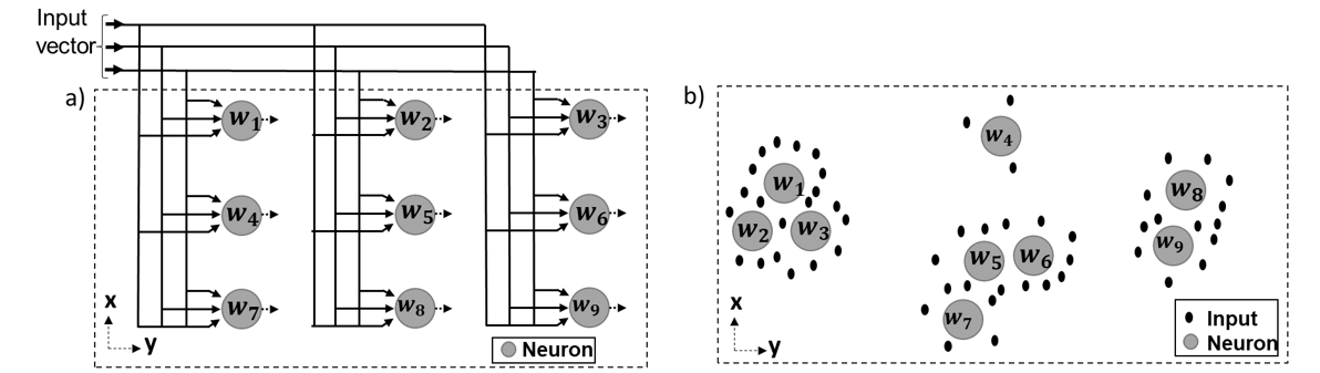
Figure 1: (a) an input vector feeding a SOM of nine neurons w1 to w9 on a 3 by 3 lattice; (b) a 2-D feature map where the nine neurons sit among clusters of input points. — **Figure 1. SOM: (a) a structure of an ANN in SOM having 9 neurons (b) the 2-D feature map of a 2-D input (example).**

The steps of the SOM algorithm for input and output spaces having the same dimensions are as following:

1. Initialization: Determine the number of neurons (i.e., $N_{w}$ ) and choose random values for $w_{i}$ ’s.

2. Sampling: Draw one sample (i.e., $u_{s} (n)$ ) from the 2-D input (i.e., u)) with a certain probability at each iteration (i.e., k).

3. Similarity matching: Find the best-matching neuron (i.e., $w_{y} (n)$ , where y is the index of the best-matching neuron) through the minimum distance criterion at the iteration k.

w_{y} (k) = arg min_{y} ‖ u_{s} - w_{y} ‖, y = 1, 2, \dots, N_{w}

(1)

4.Updating: Update $w_{j}$ ’s:

w_{j} (k + 1) = w_{j} (k) + η (k) h_{j, y} (k) (u_{s} (k) - w_{y} (k)), j = 1, 2, \dots, N_{w}

(2)

η (k) = η_{0} exp (- \frac{k}{τ_{1}})

(3)

h_{j, y} (k) = exp (- \frac{d_{j, y}^{2}}{2 ε^{2} (k)})

(4)

ε (k) = σ_{0} exp (- \frac{k}{τ_{2}})

(5)

In Eq.2, $η (k)$ is the iteration (time) dependent learning-rate parameter and $h_{j, y} (k)$ is the iteration-dependent neighborhood function. The purpose of $η (k)$ is to control the amount of the change in $w_{j}$ ’s and it is defined in Eq.3 where τ₁ is a time constant. The purpose of $h_{j, y} (k)$ is to restrict the updating procedure to the neurons that are located inside the topological neighborhood of the winning neuron (i.e., $w_{y} (k)$ ). Consequently, not only the winning neuron is updated, but the neurons around the winning neuron are updated as well. This function is defined in Eq.4, where $d_{j, y}^{2}$ is the distance between and $w_{j} (k)$ ’s and $w_{y} (k)$ and $ε^{2} (k)$ is the iteration (time) dependent width of the neighborhood function. Eq. 5 shows the formulation of $ε (k)$ where τ₂ is another time constant. Higher values of $ε^{2} (k)$ indicates larger coverage of $h_{j, y} (k)$ . Initially, almost all $w_{j}$ ’s should be included in $h_{j, y} (k = 1)$ . Values of $η (k)$ and $h_{j, y} (k)$ decrease over time as it is expected that $w_{j}$ ’s approach to the topological structure of the input space.

5. Continuation: Continue with step 2 until no change in $w_{j}$ ’s is observed.

In the IN detection method used in [1], a two-dimensional input space was created where one dimension was the value of a pixel and the second dimension was the difference of the pixel value with the median of the surrounding pixels. Then, the SOM algorithm was used to classify the corrupted and uncorrupted pixels. In this study, this approach is modified to be applicable for one-dimensional dynamic LDV signals that have similar noise characteristics as n (e.g., l). The modified method is called Modified SOM (i.e., MSOM) method. Its steps are:

First, a two-dimensional input space (i.e., $u^{l} = < u_{x}^{l}, u_{y}^{l} >$ ) of a moving LDV signal (e.g., l) is generated:

u_{x}^{l} = l - {\overline{m}}_{2 K + 1}^{l}

(6)

u_{y}^{l} = [0 0 Δ^{4} l 0 0] - {\overline{m}}_{2 K + 1}^{Δ^{4} l}

(7)

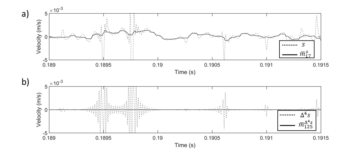
In Eq. 6, ${\overline{m}}_{2 K + 1}^{l}$ is the moving median of l. In Eq. 7, Δ⁴l is the 4^th order difference of values of l, ${\overline{m}}_{2 K + 1}^{Δ^{4} l}$ is the moving median of Δ⁴l. Two zeros are added at the beginning and the end of Δ⁴l since the fourth-order difference of a signal decrease the length of the signal by 4 points. Selection of K for ${\overline{m}}_{2 K + 1}^{l}$ and ${\overline{m}}_{2 K + 1}^{Δ^{4} l}$ are based on the length of IN observed in l and Δ⁴l. This is because the moving median is robust against artificial peaks with a length of K+1 [3]. To obtain u for s (i.e., u^s), K of ${\overline{m}}_{2 K + 1}^{s}$ and ${\overline{m}}_{2 K + 1}^{Δ^{4} s}$ were chosen as 8 and 62 since the maximum lengths of artificial peaks in s and Δ⁴s were 9 and 63, respectively. The reason of selecting a larger window size for ${\overline{m}}_{2 K + 1}^{Δ^{4} s}$ is because $s^{i_{f}}$ appear as artificial peaks in Δ⁴s due to 4^th order differentiation. Figure 2 (a) shows a segment of s and ${\overline{m}}_{17}^{s}$ while Figure 2 (b) shows a segment of Δ⁴s and ${\overline{m}}_{125}^{Δ^{4} s}$ .

Figure 2: (a) a segment of the velocity signal s and its moving median, with artificial peaks standing out of the median; (b) the fourth-order difference of s and its moving median, where the peaks appear as bursts. — **Figure 2. Signals required for $u^{s}$ : (a) a segment of s and ${\overline{m}}_{K}^{s}$ (b) a segment of Δ⁴s and ${\overline{m}}_{K}^{Δ^{4} s}$ .**

Next, create a SOM for l. Then, the points in $u^{l}$ were assigned to the closest neuron through their minimum Euclidian distance to the neuron:

C_{j}^{l (x)} = arg min_{x}_{x \in [0, N_{l}]} ‖ l (x) - w_{j} ‖, j = 1, \dots, N_{w}

(22)

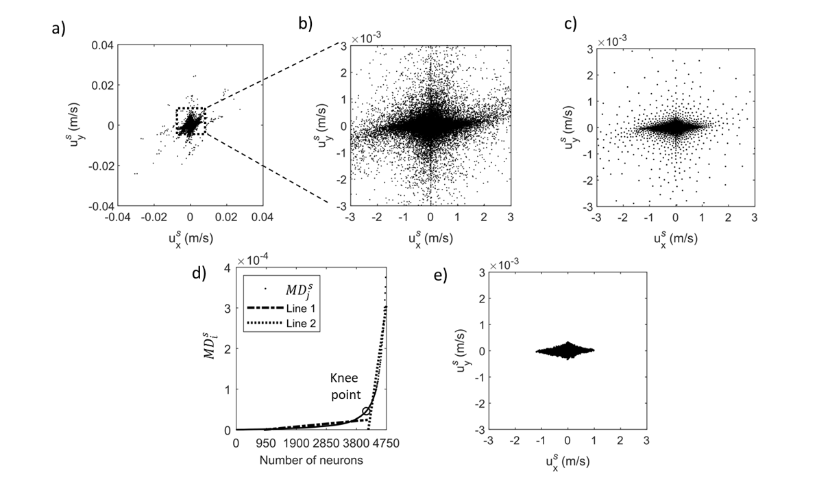
where $C_{j}^{l (x)}$ represents a signal point l(x) assigned to a neuron (e.g., w_j). A 70 by 70 two-dimensional ANN was chosen to be used in the SOM algorithm to capture the topological structure of $u^{s}$ as shown in Figure 3 (c).

Afterward, find the main trends in $u^{l}$ . To achieve this, calculate the mean of the distances between a neuron and the closest six neurons (i.e., $M D_{j}^{l}$ ). Next, sort $M D_{j}^{l}$ ’s in ascending order. Then, use the L-shape method to find the knee point [4]. Discard the points beyond this knee point. This is because some extreme points corrupt the L-shape of the curve. Then, again apply the L-shape method to the remaining points and find the second knee point. Figure 3 (d) shows the $M D_{j}^{s}$ ’s computed for s and the second knee point.

Then, find the neurons whose $M D_{j}^{s}$ values are lower than the second knee point and consider them as the neurons representing the points in $u^{l}$ that are not corrupted by IN. Figure 3 (e) shows the points in $u^{s}$ that are not corrupted by IN. The remaining points are considered to be corrupted by IN. Find their corresponding points of in l and consider them as points that are corrupted by IN.

Figure 3: scatter plots of the input space u^s (a, and zoomed in b), the neurons of the SOM spread over it (c), the sorted mean neighbour distances with the knee point where two fitted lines meet (d), and the compact cloud of points classified as uncorrupted (e). — Figure 3. The SOM classification of s: (a) $u^{s}$ (b) zoomed view of $u^{s}$ (c) the neurons of the SOM applied to $u^{s}$ (d) average of the distances between a neuron and its neighbors (e) the points classified as uncorrupted in $u^{s}$ .

H. Kong and L. Guan, “A neural network adaptive filter for the removal of impulse noise in digital images,” Neural Networks, vol. 9, no. 3, pp. 373–378, 1996, doi: 10.1016/0893-6080(95)00128-X.
S. Haykin, Neural Networks and Learning Machines. New Jersey: Pearson, 2009.
R. K. Pearson, Y. Neuvo, J. Astola, and M. Gabbouj, “Generalized Hampel Filters,” EURASIP J. Adv. Signal Process., vol. 2016, no. 1, 2016, doi: 10.1186/s13634-016-0383-6.
S. Salvador and P. Chan, “Determining the Number of Clusters / Segments in Hierarchical Clustering / Segmentation Algorithms,” in 16th IEEE International Conference on Tools with Artificial Intelligence, 2004, pp. 576–584.