 Korkut Kaynardag

Understanding Structural Health Monitoring and Nondestructive Testing: A Casual Introduction
From Vibrations to Waves: An Explanation for Newcomers
Dr. Korkut Kaynardag
Structural Health Monitoring (SHM) and Nondestructive Testing (NDT) are the practices of using sensors and data to figure out how a structure, such as a building, a bridge, a wind turbine, or an aircraft wing, is actually doing, without having to take it apart to look inside. If you have ever tapped a ceramic mug to check for a hidden crack, or had a doctor tap your knee with a small hammer to check a reflex, you have already used the same basic idea that sits underneath SHM: structures respond differently depending on their condition, and if you listen carefully enough, that response tells you something you could not see from the outside.
This article is meant as an entry point into the field: what SHM and NDT are trying to achieve, how they differ and where they overlap, how each of them actually works, why they turn out to rest on the same underlying physics even though they can look like separate fields, and what the main families of techniques are that are used to carry them out.
Why Do We Do SHM and NDT? The Three Goals
Most SHM work is aimed at one, or more, of three goals:
1. Assessing the current condition of a structure. This is the most intuitive goal: is this bridge, this building, or this wind turbine blade currently damaged, and if so, where and how badly? This is sometimes called damage detection, damage localization, or condition assessment, depending on how much detail is being asked for.
2. Monitoring a structure over the long term. A single snapshot only tells you about one moment in time. Structures are continuously loaded by operational forces, such as traffic, machinery, and people, by environmental forces, such as wind, temperature swings, humidity, and seismic activity, and, for industrial structures, by forces tied to the production process itself. Long term monitoring means keeping sensors on a structure for months or years, so that changes, whether sudden, such as an earthquake or an impact, or slow, such as fatigue, corrosion, or foundation settlement, can be tracked as they happen rather than discovered too late.
3. Updating structural models so they better reflect reality. Engineers design structures using mathematical models, most commonly finite element models, that predict how a structure should behave. But a model is always a simplification, and the real, built structure never behaves in exactly the way the model assumed. By comparing what the model predicts against what sensors actually measure, engineers can adjust, or update, the model's parameters until it matches reality much more closely. This gives a more reliable model for future predictions, including, eventually, predictions about remaining service life or how the structure would respond to a future extreme event. This kind of model updating is mostly carried out using vibration based SHM, the topic of the next section.
These three goals are related rather than separate: a good baseline model helps you detect damage, detecting damage is more useful if you are also watching it change over time, and long term monitoring data is exactly what you need to keep improving the model.
SHM and NDT Techniques
SHM shares much of its toolbox with a closely related field called NDT, short for nondestructive testing: testing that evaluates a material or structure without damaging it. Broadly speaking, SHM refers to vibration based monitoring of a structure, where the assessment is global in nature but still allows for some localization; through mode shapes, the damaged area can be narrowed down, with the resolution of that localization depending on how many measurement points are used. NDT differs from SHM in that it relies on wave propagation for pinpoint damage detection and a more detailed characterization of the damage. Putting both families together, we can group the main techniques as follows, with more detail on SHM and NDT separately following in the next sections:
Vibration based methods, the SHM approach: using how a structure moves, its dynamic response, to infer its condition.
Acoustic Emission (AE) methods, an NDT approach: listening for the sound and stress waves that damage itself produces.
Ultrasonic Testing (UT) methods, an NDT approach: actively sending high frequency sound waves into a material or structure and analyzing what comes back.
Other NDT methods: most notably eddy current testing, which uses induced electrical currents to find flaws at or near the surface of conductive materials, and X ray, or radiographic, testing, which uses penetrating radiation to reveal internal flaws, much like a medical X ray.
Eddy current testing and X ray testing work on different physical principles than the wave based methods described in this article: eddy current testing relies on electromagnetic induction, where a coil induces circulating currents in a conductive material and a flaw disturbs those currents in a way sensors can detect, while X ray testing relies on how differently a flaw absorbs or scatters penetrating radiation compared to sound material. Both are valuable, widely used techniques in their own right, but they sit outside the wave propagation story this article is actually about, so they will not be covered in much more depth here.
Before going further, it is worth explaining that Acoustic Emission and Ultrasonic Testing are best thought of as two branches of a broader family sometimes called Acoustic Testing: both rely on the exact same underlying elastic wave physics, just pointed in opposite directions, and it is worth being precise about the difference, since the terms get used loosely. Acoustic Emission (AE) is a passive technique: sensors simply listen, in real time, for the tiny stress waves that a structure releases on its own when something happens inside it, such as a crack growing or a fiber snapping. Ultrasonic Testing (UT), by contrast, is an active technique, where a probe, or probes, deliberately sends a high frequency wave pulse into the material, and sensors analyze the reflected or transmitted signal to find defects, the same way sonar works. Both rely on the same underlying wave physics, which is why they are grouped together in the explanation below, but they answer slightly different questions: AE tells you that damage is happening right now, somewhere; UT tells you whether a specific location currently contains a flaw. Both are covered in more detail further below.
The rest of this article focuses on the two families known best from my own research: vibration based SHM, and wave propagation-based methods, meaning acoustic and ultrasonic testing.
Vibration Based Monitoring (SHM): Listening to the Whole Structure
Every structure has a natural way it prefers to vibrate. Push it, or let the wind, traffic, or an earthquake push it, and it will oscillate most strongly at a handful of specific frequencies, called resonance frequencies or modal frequencies. This is the same phenomenon that lets an opera singer shatter a wine glass by matching their voice to the glass's natural frequency, or lets you get a swing moving higher and higher by pushing it at just the right moments.
Three parameters are typically extracted from this vibration behavior:
Modal, or resonance, frequencies: the specific frequencies at which the structure vibrates most strongly.
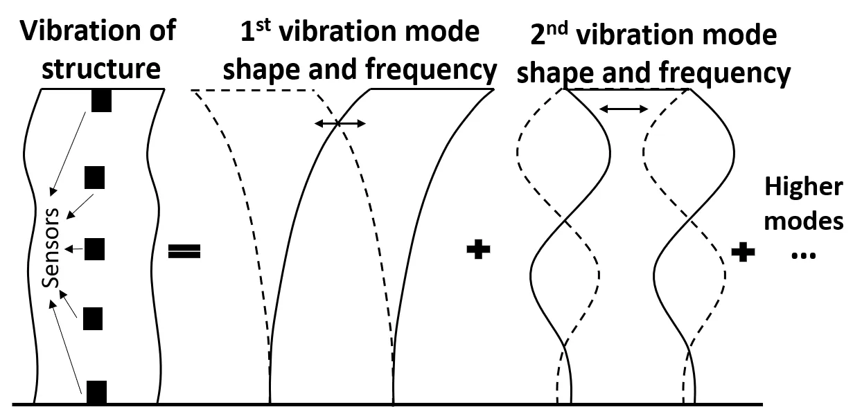
Mode shapes: the pattern of that vibration at each resonance frequency. For example, a beam's first mode might look like one smooth bump, while its second mode looks like the letter S, with a stationary point in the middle.
Damping ratio: how quickly the vibration dies out once the exciting force stops, a measure of how efficiently the structure dissipates energy.
These are called global vibration parameters, see Figure 1, because they describe the behavior of the structure as a whole, and they typically occur at relatively low frequencies, often well under 100 Hz for large civil structures like buildings and bridges, though they can reach a few kHz for very rigid, small structures, such as a short length of rail track supported between two sleepers.
How Damage Shows Up
Damage, such as a crack, a loosened connection, corrosion, or foundation movement, changes a structure's stiffness or mass distribution. Since resonance frequencies, mode shapes, and damping all depend on stiffness and mass, damage leaves a fingerprint on all three. Condition assessment, then, largely comes down to comparing a structure's current vibration parameters against a baseline, either measurements taken when the structure was known to be undamaged, or the predictions from a finite element model of the intact structure, and looking for meaningful changes.
That same comparison, run in reverse, is how finite element, or analytical, model updating works: rather than assuming the model is correct and looking for changes in the real structure, engineers adjust the model's parameters, such as material stiffness, boundary conditions, and mass distribution, until the model's predicted dynamic properties come out as close as possible to the ones actually measured on the real structure. Long term monitoring typically supports both of these efforts at once, condition assessment and model updating, by keeping instrumentation on a structure over an extended period and repeating the comparison as new data comes in.
How the Measurements Are Actually Taken
To capture global vibration behavior, sensors called vibration transducers, most commonly accelerometers, are attached to the structure. Measurement without any contact is also possible, most notably with a Laser Doppler Vibrometer, which reads vibration directly off the structure's surface without ever touching it. The recorded signals are then run through system identification algorithms to extract the resonance frequencies, mode shapes, and damping ratios.
There is an important fork in the road here, depending on whether you know the force that is shaking the structure:
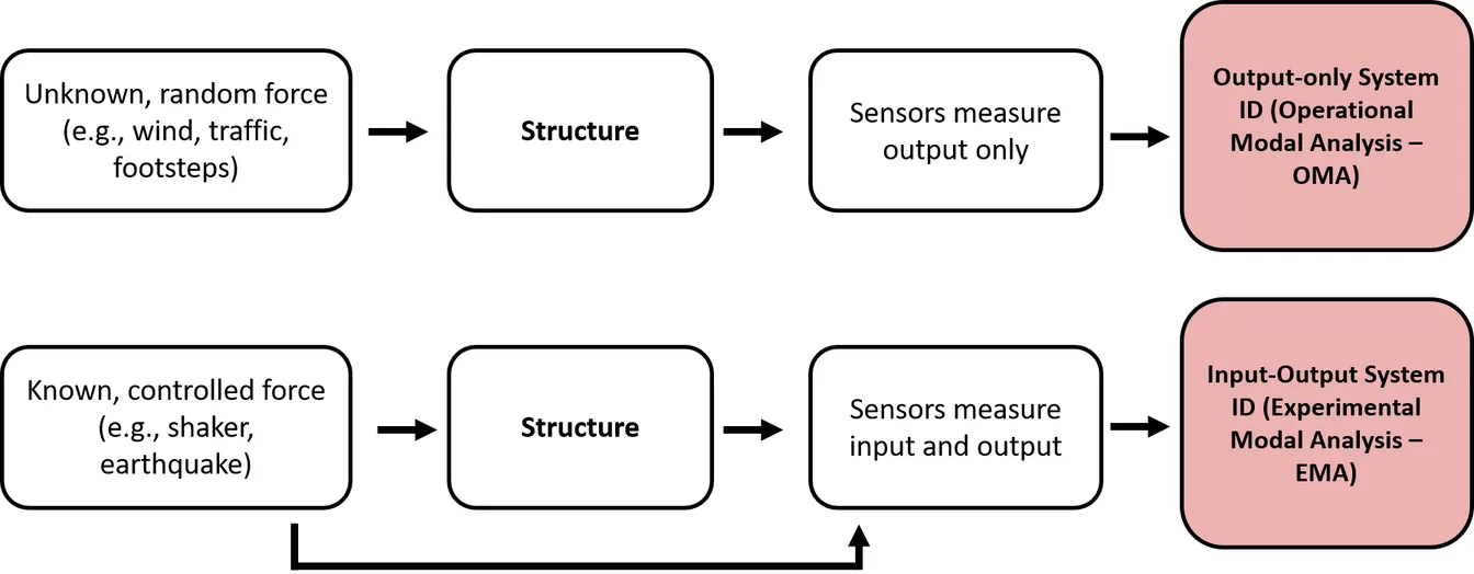
In most real world civil structures, the forces causing the vibration, such as wind gusts, people walking, passing traffic, or running machinery, are essentially random and unmeasured. In this case, engineers and researchers use system identification methods based only on the measured output, a branch of the field often called Operational Modal Analysis, or OMA, which can extract modal parameters from the vibration response alone, without ever knowing the exact input force.
When the input force is known and controlled, for example a structure excited in a laboratory with a calibrated modal shaker, or the ground motion recorded at the base of a building during an earthquake, engineers and researchers can instead use system identification methods based on both the input and the output, often called Experimental Modal Analysis, or EMA, which tend to give cleaner, more precise results because both the cause and the effect are known. See Figure 2 for the OMA and EMA workflows.
For model updating, whichever route gets you there, the resulting resonance frequencies, mode shapes, and damping ratios are exactly the quantities that feed the model updating process described above. The analytical or finite element model is adjusted until it reproduces these same measured properties as closely as possible.
Doing this well is genuinely interdisciplinary. A solid grasp of signal processing, to make sense of noisy, real world data, of optimization algorithms, and of probability and statistics, since many system identification and model updating methods are fundamentally optimization or statistical inference problems, is essential. Structural dynamics is essential too, both for understanding the dynamic behavior itself and for the model updating side specifically. In recent years, neural networks and machine learning have also been applied throughout this pipeline, to improve automated damage detection, reduce noise in the measured signals, and make finite element model updating faster and more robust.
Within the SHM and NDT field, this type of monitoring is usually just called SHM, which is why only SHM appears in this section's title.
Wave Propagation Based Monitoring (NDT): Listening to One Spot Closely
While vibration based SHM asks how the whole structure is behaving, wave propagation methods ask a more zoomed in question: is there a flaw right here? In this case, the quantity of interest is essentially how a wave scatters, reflects, and transmits as it interacts with defects and boundaries.
The underlying idea is the same one bats use to navigate in the dark, sending out a sound pulse and reading the timing and shape of its echo, the reflection from surrounding surfaces, to sense what is around them. Another everyday example is the ultrasound scan your doctor might use. In our case, high frequency waves are sent into a material, and because waves reflect off boundaries and discontinuities, including cracks, delaminations, corrosion pits, and voids, the reflected and transmitted signal carries information about what is inside. These waves generally travel at much higher frequencies than the global vibrations described earlier, typically in the kilohertz to megahertz range, which is part of why they are so good at picking out small, localized flaws rather than describing the structure as a whole.
Processing these signals mostly comes down to feature extraction: probes send out a wave with a known, specific shape, and signal processing techniques, matched filtering and correlation based methods being common choices, are used to identify that same shape, along with its arrival time and amplitude, buried inside the noisy recorded signal, filtering out the unwanted noise that inevitably creeps into real world measurements. As with vibration based SHM, neural networks and machine learning have increasingly been applied here too, both to suppress noise and to automatically classify the patterns that damage leaves behind in the recorded signals.
From a Single Reading to a Full Picture
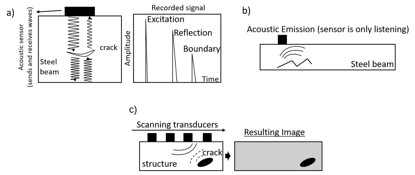
A single probe sending and receiving one wave only tells you about the material directly along that one path, though since sound can propagate in many directions, monitoring along multiple paths at once also works. This is done either by sending waves and sensing the reflections, which is ultrasonic testing, see Figure 3a, or by only listening to the structure over time, which is acoustic emission testing, see Figure 3b. This is useful, but limited, a bit like checking a patient's pulse at a single point on their wrist. Imaging takes ultrasonic testing further: instead of one probe, an array of transducers sends waves along many different paths through the structure and records all of the reflections. Combining all of these individual readings together, much like a medical CT or ultrasound scanner builds a full picture from many individual passes, lets engineers reconstruct an actual internal view of the structure, showing not just whether a flaw exists, but its shape, size, and location, see Figure 3c. This is still a form of ultrasonic testing, just using many probes instead of one.
Bats are a nice everyday analogy for all three cases. A single echolocation pulse from a bat, bouncing off one obstacle, is essentially the pulse echo case of ultrasonic testing, shown in Figure 3 (a). A bat hearing a nearby branch crack is a good analogy for acoustic emission, shown in Figure 3 (b). And a bat's brain combining many echoes from its own calls into a single picture of its surroundings is closer in spirit to the imaging case in Figure 3 (c), though in our case, we are the ones sending all the waves.
Accordingly, this second broad approach, wave propagation monitoring, is usually referred to as NDT, though in practice SHM and NDT are often used interchangeably as well. Later in this article, two specific kinds of waves used in NDT, guided waves and bulk waves, are covered in more detail.
How SHM and NDT uses actually same physics – wave propagation: An Explanation Based on My Own Experience
Here is where I want to share something that genuinely confused me for a while, because I suspect it confuses a lot of people coming into this field the way I did.
My MSc research was in vibration based SHM, the low frequency, whole structure world. My PhD research was in NDT, the high frequency, localized wave propagation world. Working across both, I kept treating them as two separate toolkits for two separate problems. But they are not separate at all: the low frequency resonance modes of a structure are themselves a product of wave propagation. Vibration based SHM is not an alternative to wave physics, it is a special case of it.
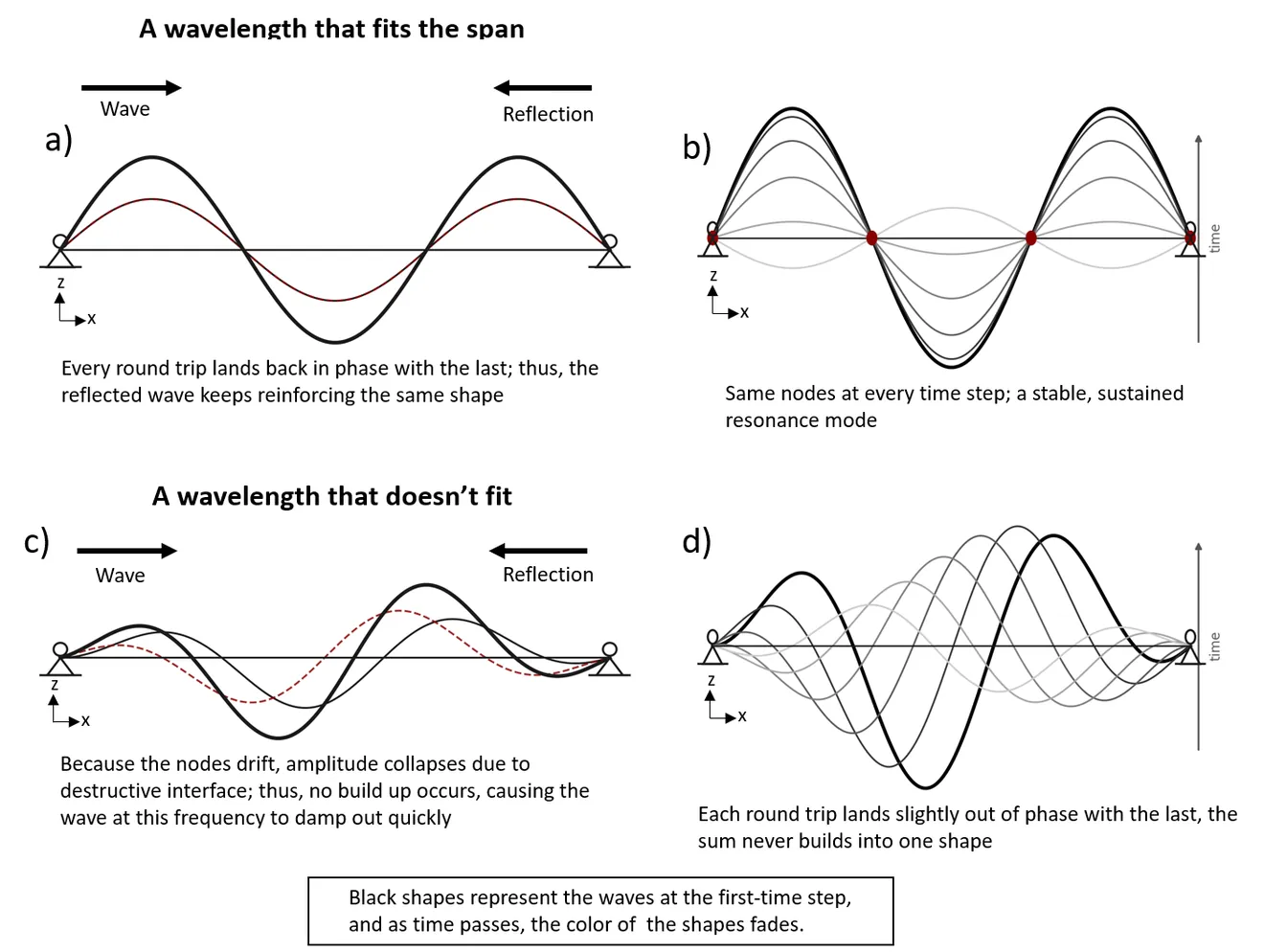
Here is the intuition. Imagine a guitar string, fixed at both ends. When you pluck it, you are not creating one wave that travels in a single direction forever: you are creating waves that travel down the string, hit the fixed end, and reflect back. Very quickly, you have waves traveling in both directions at once, overlapping and interfering with each other, as shown in Figure 4 (a). For a special set of wavelengths, specifically the ones where an integer number of half wavelengths fits exactly into the length of the string, the two opposing traveling waves interfere constructively in a very particular, stable pattern: a standing wave, where some points barely move at all, the nodes, while others swing back and forth with maximum amplitude, the antinodes, as shown in Figure 4 (b). For most other wavelengths, the two traveling waves interfere destructively instead: their peaks and troughs do not consistently line up, so the combined vibration stays small and dies out quickly rather than building into a stable pattern, as shown in Figure 4 (c) and 4 (d).
That standing wave is, physically, exactly what we call a resonance mode. The wavelength that produces it determines the resonance frequency; the pattern of nodes and antinodes is the mode shape. Scale this idea up from a guitar string to a beam, a floor slab, or an entire building, and the principle does not change: what looks like the building swaying at its natural frequency is, underneath, the same reflect and interfere process that produces the localized waves used in ultrasonic testing, just happening at a much lower frequency, over the full length of the structure, with reflections bouncing off the structure's own boundaries and supports rather than off a crack.
These ideas, the standing waves, the reflections, the mode shapes, have all been illustrated using beams as the running example, mostly because a beam's geometry is the simplest one to sketch and reason about. The same underlying logic carries over to other shapes of structure, though: a plate or shell supports waves traveling in two directions instead of one, often called Lamb waves, and a pipeline's thin, curved wall guides its own family of wave modes along its length and around its circumference. The bookkeeping gets more involved, with more possible wave modes and more geometry to track, but physics does not change. It is still reflection and interference, and resonance is still just a standing wave that fits the boundaries exactly.
Because a resonance mode's frequency, shape, and damping are all extremely sensitive to a structure's stiffness, mass, and boundary conditions, it is rarely useful in practice to think about vibration based SHM in terms of individual traveling waves. Treating the resonance modes themselves as the parameters of interest, as described earlier, is simpler and works just as well. But it is worth understanding why that shortcut works, rather than treating the two branches of SHM as unrelated fields that just happen to share some vocabulary. It matters for another reason too: resonance modes are also central to how engineers calculate a structure's dynamic response in the first place. I spent a long time wondering how the equations of motion actually produce these frequencies and shapes, and this wave picture is what finally made it click for me.
There is a nice real world example of the two worlds meeting directly: earthquakes generate relatively low frequency waves that propagate up through a building from its base. Instead of only asking how the building's resonance frequencies, mode shapes, or damping changed after the earthquake, the classic vibration based SHM question, some researchers instead study how that low frequency wave itself traveled and changed as it moved up through the structure, using techniques that are conceptually much closer to the wave propagation methods used in NDT. It is the same underlying physics, approached from the other direction.
Guided Waves and Bulk Waves: Two Ways NDT Sends a Wave
Here, I will explain the wave types that are used in NDT, as I explained above how vibration based SHM also uses wave propagation in terms of modal frequencies and shapes.
That same reflect and interfere logic also explains something specific to NDT itself: why a high frequency wave behaves differently depending on how high its frequency actually is. As frequency increases, wavelength decreases, and the wave becomes more localized within the cross section of whatever it is traveling through. The bending waves used in the guitar string and beam example above operate at relatively low frequencies and engage the whole cross section as they travel. At higher frequencies, the wave modes, called guided wave modes, start to behave more like the resonant, standing wave pattern just described, but across the thickness of the part rather than along its whole length: their speed depends on frequency, a property called dispersion, and at sufficiently high frequency they decouple into waves confined near the top surface, the bottom surface, or another specific region of the cross section. Because these higher frequency waves have much smaller wavelengths, they can interact with small defects, which is what makes them useful for NDT.
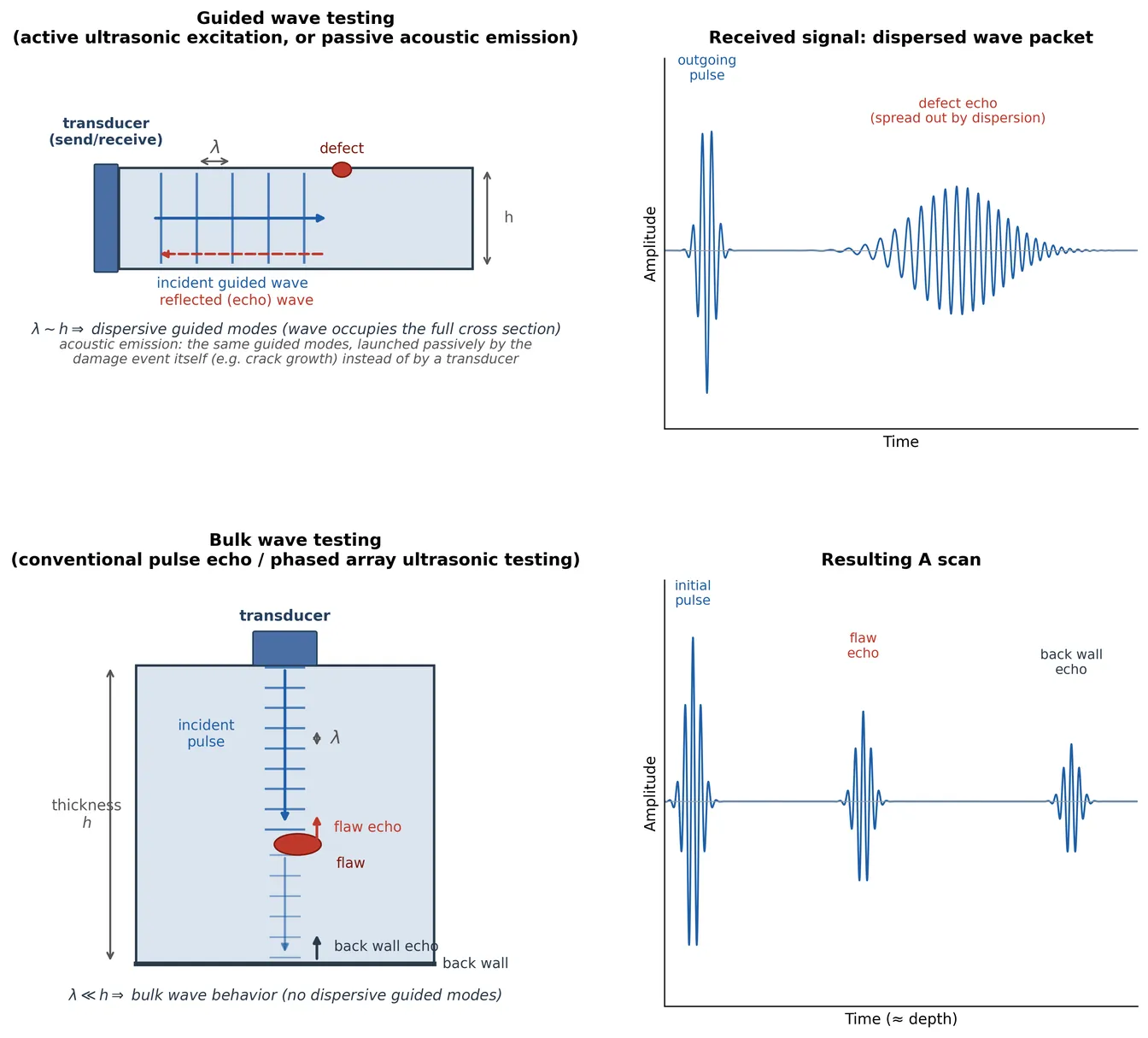
These guided wave modes are what both acoustic emission and guided wave ultrasonic testing rely on, shown on the left in Figure 5. In guided wave ultrasonic testing, a transducer actively sends a wave along the length of the structure, using the full thickness as a waveguide, so a single sensor pair can interrogate a long stretch or a wide area rather than just the point directly beneath it. Acoustic emission relies on the same guided modes, but passively: instead of a transducer sending the wave, the damage event itself, such as crack growth or fiber breakage, releases energy that launches these guided modes at the source, and they propagate outward to the sensors without any external excitation. Because the wavelength is comparable to the thickness in both cases, the wave is dispersive, so the signal that arrives at the sensor tends to be spread out in time rather than arriving as a single sharp pulse.
Ultrasonic testing can also be carried out without relying on this behavior, which depends on the cross section, at all, shown on the right in Figure 5. When the wavelength is small relative to the part's thickness, the wave no longer interacts with the boundaries strongly enough to set up dispersive guided modes, and instead behaves essentially as it would in an infinite medium, reflecting off flaws and back walls in a straightforward way. This is the basis of conventional bulk wave ultrasonic testing, such as pulse echo or phased array scanning, which builds up an image point by point rather than requiring interpretation of dispersive mode behavior. In practice, arrays with many elements are generally used with bulk waves, since steering and focusing the beam for point by point imaging depends on this simple propagation, which does not spread out the way guided waves do. A single probe, on the other hand, can go either way: conventional bulk wave pulse echo, or, at lower frequency, excitation of guided wave modes for inspection over long distances.
Thus, we can say: acoustic emission testing is guided wave based, single probe ultrasonic testing is guided wave and bulk wave based, and multi-probe ultrasonic testing is usually bulk wave based (while some examples exist using guided waves for long range inspection).
Putting It Together
If you are new to SHM, the main things worth carrying away are these. The field exists to answer three practical questions: is this structure currently damaged, how is it changing over time, and how can our models of it get more accurate. It answers them using two broad physical strategies. One strategy steps back and studies the structure's overall vibration behavior, comparing it to a healthy baseline. The other strategy zooms in and sends high frequency waves through a specific region, listening for what bounces back. They can feel like entirely different fields when you are learning them separately, the way I did. But at their core, they are both just different ways of listening to how waves move through a structure, and to what those waves reveal about the material they have traveled through.