 Korkut Kaynardag
Understanding Sound Classification, Localization and Tracking and Similarity to NDT
Dr. Korkut Kaynardag
You've probably started to notice a lot of smart devices lately that only have microphones, yet can identify what kind of sound they're hearing, and in some cases even track where it's coming from. This is something I worked on in my career, and it's actually closely related to non-destructive testing (NDT): many of the same underlying signal processing, noise reduction, angle of arrival and localization, tracking and pattern recognition algorithms show up in both fields. In NDT, such algorithms are applied to sound waves propagating in solids that are recorded from the structures, while in this case, they are applied to sound waves propagating in the air. Here I'll explain how these systems generally work. (I will talk about vibration based structural health monitoring, i.e., SHM, at the end of the document)
Three Main Stages
1. Sound Detection. Machine learning (ML) methods are used to decide whether a sound of interest is present at all, and if so, what kind of sound it is (a dog barking, glass breaking, a particular voice, and so on). Models are trained on large libraries of labeled recordings so that they can learn to recognize the distinctive pattern each sound type produces. Conventional, non-neural network ML classifiers work from features computed on the time-domain signal itself (things like zero crossing rate and short-time energy) as well as from their frequency-domain transformations (spectral centroid, spectral roll-off, and coefficients such as MFCCs), while neural network-based methods usually skip hand-crafted features and work directly from spectrograms or mel spectrograms. A typical pipeline slides a short analysis window for real-time processing, often tens of milliseconds long, across the incoming audio stream and produces a classification decision for each window; these frame-level decisions are then smoothed over time, often with a simple majority-vote or median filter over a few consecutive windows, so the output does not flicker between classes. It is also worth separating two related tasks: sound classification, where the goal is just to label a fixed clip, and sound event detection, where the goal is to also mark when each event starts and ends within a continuous stream.
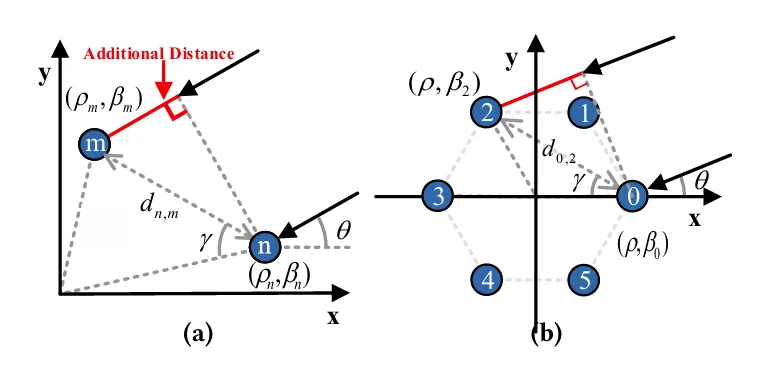
2. Sound Direction Estimation/Localization. Linear or circular microphone arrays are used here: because sound reaches each microphone in the array at a very slightly different time (phase difference) and with a slightly different level, comparing these small differences across the microphones in the array configurations lets the system estimate the direction the sound is arriving from. There are localization and angle of arrival (AoA) algorithms specifically tailored to such applications. Two families dominate here. Time difference of arrival methods, such as generalized cross correlation with phase transform, estimate the small delay between each pair of microphones and convert it directly into an angle. Subspace-based methods, such as MUSIC, instead build a statistical model of the incoming signal and search for the direction that best explains the correlations observed across the array; these tend to be more accurate but also more demanding computationally. Much simpler algorithms with better computational efficiency also exist. Array spacing matters as well: if the distance between microphones is too large relative to the wavelength of the sound being tracked, the array becomes ambiguous about direction, an effect known as spatial aliasing, so the geometry has to be matched to the frequency range of interest. A related, more direct technique is delay-and-sum beamforming, which simply time-shifts and adds the signals from each microphone so they reinforce each other for a chosen look direction while other directions partially cancel out, the same array can then be electronically “steered” toward a source, or away from a known noise source, without physically moving it. Figure 1 (a) shows how a pair of linear array sensors determines the direction of a sound wave's arrival from the additional distance traveled to sensor m. However, considering 180-degree symmetry, this case can't separate which of the two 180-degree sides the wave is coming from. To overcome this, more sensors are placed in a circular pattern as the sound will arrive at different times to each mic no matter which direction it is coming from in a 360-degree plane, as in Figure 1 (b). Full sound-source localization works similarly, but also incorporates reflections in the analysis, since multipath returns can help recover a source's actual position, not just its bearing.
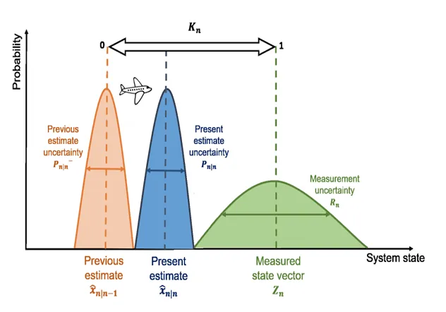
3. Sound Target Tracking. A single direction estimate is just a noisy snapshot in time, so Kalman filters are used to combine incoming estimates with a model of how the source is expected to move, producing a smoothed, continuously updated track of the source’s location. The filter alternates between two steps. In the predict step, it uses a motion (process) model that is expressed as a set of linear equations in matrix form to project the current state estimate forward in time, producing a predicted location for the next measurement together with an updated uncertainty (variance) for that prediction. In the update step, this prediction is combined with the actual incoming measurement, which carries its own uncertainty based on the local signal statistics, signal-to-noise ratio, and other similar features. Because both the predicted state and the new measurement are represented as probability distributions with a mean and a variance, they can be combined into a new, more precise estimate using a weighting term called the Kalman gain: when the measurement is noisy relative to the model, the gain is small and the filter leans more on its own model-based prediction; when the model is uncertain relative to the measurement, the gain is large and the filter trusts the incoming measurement more. This predict-update cycle is the basic core idea of Kalman filters. Figure 2 illustrates how this approach works statistically: the previous estimate and its uncertainty are propagated forward into a present (predicted) estimate, which is then fused with the uncertain measurement to produce an updated estimate whose variance is smaller than either input on its own. In its simplest form the filter assumes the source moves smoothly, so a constant velocity or constant acceleration model is often enough; when the motion is more erratic, an extended or unscented Kalman filter, or a particle filter, is used instead to handle the nonlinearity. A separate, often underrated problem is data association: when more than one sound source is active at once, the tracker first has to decide which new measurement belongs to which existing track before it can even run the filter update, and mistakes at this stage tend to cause tracks to swap or merge.
Other Components
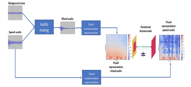
Noise Reduction: removing sounds that are not of interest, so the sound of interest can be enhanced before the stages above are applied. This is based on signal processing and machine learning methods, much like the detection stage itself. This is a big research topic, and the internet is rich with articles related to it. Classical approaches include spectral subtraction and Wiener filtering, which estimate the noise spectrum during quiet periods and subtract it from the incoming signal, and adaptive beamforming, which reuses the same microphone array from the localization stage to steer a spatial null toward known noise sources. More recently, neural networks trained on pairs of clean and noisy recordings have become the dominant approach, since they can learn noise patterns that are hard to describe with a simple formula. Figure 3 shows one such approach: a variational autoencoder (VAE) trained to remove background noise from a speech signal. As shown in Figure 3, background noise and clean speech audio are each sourced separately and then mixed together to build the training pairs the network needs: a noisy spectrogram as input, and the clean spectrogram it should reconstruct as the target. This is feasible as background noise is simply an addition to a clean signal of interest (speech in this case). During training, the VAE's encoder compresses the noisy spectrogram into a compact latent representation, and its decoder reconstructs a clean spectrogram from that representation; the network is optimized to minimize both the reconstruction error against the true clean spectrogram and a KL-divergence term that keeps the latent space well-structured, so that at inference time the decoder generalizes to noise conditions it has not seen in exactly that form before. Once trained, the model is used purely in a feed-forward manner: a new noisy recording is converted to a spectrogram, passed through the encoder and decoder, and the resulting denoised spectrogram is converted back into a waveform with an inverse STFT to produce the enhanced output. Moreover, sound detection or classification now can be applied on the cleaned STFT spectrogram for more reliable results. Unlike the classical methods above, this approach requires a training dataset of paired noisy/clean examples up front, but in exchange it can learn noise characteristics that are difficult to capture with a fixed formula, at the cost of needing enough representative training data to generalize to real-world noise conditions. (Nogales, A., Caracuel-Cayuela, J., & García-Tejedor, Á. J. (2024). Analyzing the influence of diverse background noises on voice transmission: A deep learning approach to noise suppression. Applied Sciences, 14(2), 740).
Distance Estimation: once the direction of a sound is known, it is often also useful to know how far away it is. This is a harder problem, since distance is not as directly encoded in the signal as direction is, but it is commonly approached by tracking how the sound’s amplitude decays as it travels, in free field conditions, sound pressure falls off roughly 6 dB for every doubling of distance from the source, or, when the type of source is well known, through time-of-flight or time-of-arrival-style techniques. Amplitude-based estimates are cheap to compute, but they are easily thrown off indoors, where reflections off walls and furniture add energy back into the signal well after the direct path has already decayed. Where two or more separated microphone arrays are available, distance can also be recovered geometrically, by triangulating the direction estimates from each array, in much the same way a surveyor fixes a position from two bearings.
Wrapping Up
Here, we explained how a sound source or multiple sound sources can be detected, how their arrival direction or full location can be estimated, and how they can be tracked over time. Very similar algorithms are also used in NDT, to determine the type and location of a defect inside a structure. Very fun topics and analysis 😊
The Kalman filter we used for sound tracking is a good example of this crossover. In guided-wave and acoustic-emission based NDT, the same predict/update framework is used to localize and track a defect: instead of a sound source's position, the "state" being estimated is the defect's location (and sometimes its severity), and instead of microphone time-delay measurements, the inputs are the times of arrival or amplitudes of elastic waves recorded at multiple sensors. As new wave packets arrive, the filter fuses each new measurement with the model's prediction, refining the location estimate and smoothing out sensor noise, the same way it smooths a moving sound source's trajectory. Kalman filters (and their nonlinear variants, such as the extended Kalman filter) are also used more broadly in vibration based structural health monitoring (SHM) to track parameters that change over time, for example, tracking a structure's stiffness as it degrades during an earthquake or a fatigue test, or tracking a bridge's neutral axis position as it shifts with temperature. In all these cases, the appeal of the Kalman filter is the same: it is a computationally efficient way to combine an imperfect model with noisy, streaming measurements and get a running best estimate, whether what's being tracked is a moving sound, a growing defect, or a slowly changing structural property.
System identification, which we mentioned briefly earlier in the context of vibration-based SHM, follows this same theme of extracting hidden information from measured data, just applied to an entire structure instead of a sound source or a defect. Given vibration data recorded from sensors on a structure, system identification methods estimate its modal parameters, natural frequencies, mode shapes, and damping ratios, by treating the structure itself as an unknown system to be identified from its input (if measured) and output (always measured) signals. When only the structure's response is available and the excitation is not measured directly, such as under ambient traffic or wind loading, output-only methods are used; the most common ones include the Frequency Domain Decomposition (FDD) method, which identifies modes from peaks in the singular values of the response's power spectral density, and Stochastic Subspace Identification (SSI), which works directly in the time domain and tends to give more accurate and better-separated modal estimates, especially for closely spaced modes. When both the input excitation and the output response are available, such as from a hammer impact or shaker test, methods like the Eigensystem Realization Algorithm (ERA) can be used instead. For structures whose properties change over time, whether gradually, like a bridge's stiffness drifting with temperature, or suddenly, due to damage, recursive versions of these methods (such as recursive SSI) or Kalman-filter-based identification schemes are used to track the modal parameters online, updating the estimate as each new batch of data comes in rather than waiting to reprocess the entire dataset from scratch.
Taken together, sound detection and tracking, defect detection and tracking in NDT, and system identification in vibration-based SHM are really different applications of the same underlying idea: using noisy, streaming sensor data together with a model of how the underlying system behaves to estimate something that cannot be measured directly, whether that is a sound source's position, a crack's location inside a structure, or a bridge's natural frequencies.
Sources: